Implementation Techniques Targeting Hardware ... - Semantic Scholar

Model-driven Engineering from Modular Monadic Semantics: Implementation Techniques Targeting Hardware and Software? William L. Harrison1 , Adam M. Procter1 , Jason Agron2 , Garrin Kimmell3 , and Gerard Allwein4 1

2

Department of CS, University of Missouri, Columbia, Missouri, USA Department of CS & CE, University of Arkansas, Fayetteville, Arkansas, USA 3 Department of EECS, University of Kansas, Lawrence, Kansas, USA 4 US Naval Research Laboratory, Code 5543, Washington, DC, USA

Abstract. Recent research has shown how the formal modeling of concurrent systems can benefit from monadic structuring. With this approach, a formal system model is really a program in a domain specific language defined by a monad for shared-state concurrency. Can these models be compiled into efficient implementations? This paper addresses this question and presents an overview of techniques for compiling monadic concurrency models directly into reasonably efficient software and hardware implementations. The implementation techniques described in this article form the basis of a semantics-directed approach to model-driven engineering.

1

Introduction

System software is notoriously difficult to reason about—formally or informally— and this, in turn, greatly complicates the construction of high assurance systems. This difficulty stems from the conceptual “distance” between the abstract models of systems and concrete system implementations. Formal system models are expressed in terms of high-level abstractions while system implementations reflect the low-level details of hardware, machine languages and C. One recent trend in systems engineering—model-driven engineering (MDE) [40]—attempts to overcome this distance by synthesizing implementations directly from system specifications. The MDE methodology is attractive for high assurance applications because the process proceeds from a domain specific modeling language that, when specified with a suitable formal semantics, will support verification. The starting point for this work is recent research applying modular monadic semantics to the design and verification of trustworthy concurrent systems [15, 14, 12, 13]. There are a number of natural “next” questions concerning the set of design and verification principles developed in the aforementioned publications. ?

This research was supported by NSF CAREER Award 00017806; US Naval Res. Lab. Contract 1302-08-015S; DARPA/AFRL Contract FA8650-07-C-7733; the Gilliom Cyber Security Gift Fund; Cadstone, LLC; and the ITTC Tech. Transfer Fund.

2

Can system implementations be generated from monad-based specifications and, if so, how is this best accomplished? Are critical system properties preserved by implementation techniques? Can acceptable performance across many dimensions (including speed, size, power consumption, etc.) be achieved? This paper addresses the first question and leaves the others to future work. This paper considers an instance of MDE for which the models are based in the modular monadic semantics (MMS) of concurrent languages [12, 34]. Monads have a dual nature, being both algebraic structures with properties and a kind of domain-specific language (DSL) supporting programming. The view of monads as DSLs is just the standard view within the functional programming community expressed in a non-standard way: monads encapsulate a specific flavor of computation and provide language constructs (i.e., monadically-typed operators) in which to build computations. The contributions of this paper are: (1) An exploration of the design requirements for a monadic DSL for describing small concurrent systems with shared state (e.g., embedded controllers). This language is called Cheap Threads after an article of the same name [18]. (2) Implementation techniques for Cheap Threads (CT) programs targeting both a fixed instruction set and hardware circuits. The first technique is a traditional compiler for a non-traditional language. The second technique translates a CT program into VHDL code from which circuitry may be synthesized and loaded into an FPGA. A DSL for specifying state machines called FSMLang [3] serves as an intermediate language. (3) A significant case study demonstrating the application of these techniques to the automatic generation of software-defined radios [23] from CT-style specifications. It is sometimes said of domain specific languages that what is left out of them is more important than what is left in. By restricting its expressiveness, a DSL design can better capture the idioms of its targeted domain. This is just as true in our case where the limitations imposed are intended to aid in the ultimate goal of verifying high assurance properties. Both with respect to its semantics and implementation strategies, what is left out of CT is crucial to the success of this approach. Because the semantics of CT is fundamentally simpler than that of Haskell, its implementation can be made far simpler as well. Although it dispenses with the constructs that complicate Haskell 98’s semantics, CT retains the necessary expressiveness—but no more expressiveness than is necessary. The decision to create a standalone CT language (as opposed to an embedding within a language such as Haskell) was made for the sake of semantic simplicity. Haskell 98 [36], for example, has a surprisingly complicated semantics [17, 21, 11] due to certain of its features (e.g., the seq operator, expressive pattern-matching, polymorphic recursion and type classes), while its extension, GHC Haskell, has no standard semantics at all. Furthermore, excluding features such as general recursion results in much more predictable time and space behavior. CT possesses a built-in semantics as each CT language construct corresponds to an algebraic operator of a fixed monad. Syntactically, CT is simply a sublanguage of Haskell, extended with a simple declaration form for specifying monads. Any CT program is also a Haskell pro-

3

gram that can be executed with standard implementations like GHC or Hugs. CT contains only the small core of Haskell 98 necessary for defining computations within these monads (function and data declarations, etc.). In particular, CT dispenses with first-class functions, curried functions and partial application, recursive data structures, type classes, polymorphism, the IO monad, and much of the complexity of Haskell 98’s pattern matching. General recursion is eschewed in favor of an explicit fixed point operator which operates only on tail-recursive functions. Another reason to define CT as a standalone language is that, as it will be independent of Haskell implementations, the ultimate results of this research can be re-used far more readily in a variety of settings. There is no high assurance run-time system for Haskell, so relying on the GHC run-time, for example, just “kicks the high assurance can down the road.” For embedded systems and many varieties of system software (e.g., garbage collectors, network controllers, device drivers, web servers, etc.), the size of the object code produced would have to be small to be practical, thus eliminating all current Haskell implementations. The presence of garbage collection in Haskell run-time systems is completely unacceptable for some software systems because of timing issues (e.g., flight control software). It is fortunate, therefore, that CT does not require the full power of the Haskell RTS with its attendant unpredictable time and space behavior. When considered individually, software compilation and hardware synthesis represent signal achievements in Computer Science. While there has been some success with mixed target compilation—i.e., the generation of either hardware or software implementations from a single source—the record is mixed. The challenge derives in trying Register to compile the same specification Transfer Xilinx Language Cheap MicroBlaze into targets—i.e., hardware and Threads FPGA FSMLang software—that encapsulate vastly DSL different notions of computation. The use of monads in the present work allows us to explicitly tailor the source notion of computation so that it may be implemented efficiently in either hardware or software. The implementation techniques considered here are portrayed in the inset figure. The Cheap Threads language is defined in Section 3. The top route (described in Section 4) shows what is essentially a traditional compiler for a non-traditional language producing RISC MicroBlaze machine language. The lower path (described in Section 5) first generates an intermediate form in FSMLang, which is a DSL specifying for abstract state machines. FSMLang provides a clean target for synthesis at a lower level of abstraction than CT and can be readily translated into a netlist for the Xilinx FPGA. The rest of this section presents related work and Section 2 presents an overview of monadic semantics and defunctionalization. Section 6 presents a case study in the application of Cheap Threads to the specification and implementation of software defined radios. Section 7 presents conclusions and future work. Related Work. Recent research concerns the construction and verification of formal models of separation kernels using concepts from language semantics [15,

4

14, 12]. These models may be viewed as a domain-specific language (DSL) for separation kernels and can easily be embedded in the higher-order functional programming language Haskell 98 to support rapid prototyping and testing. The “by layer” approach to implementing monadic programs—i.e., compiling by monad transformer—was first explored by Filinski [9] who demonstrated how the most commonly used layers (i.e., monad transformers) may be translated into a λ-calculus with first-class continuations; the resulting program could be then further compiled in the manner of Appel [5]. Filinski’s approach would work here as it handles all of the monad transformers used in CT. Li and Zdancewic [26] show how a monadic language of threads may be implemented via the GHC compiler; their implementation is efficient with respect to execution speed. Their work is not intended to provide efficiency with respect to code size as is ours. Liang and Hudak [27] embed non-proper morphisms of a source monadic expression in Standard ML, thereby providing a means of implementing monadic programs. We opted for a more standard approach to compilation than these as doing so would give more control over the target code produced and, furthermore, seemed more susceptible to verification. Recent research applies DSLs to bridge the distance between the abstract models of systems and concrete system implementations. DSLs targeting the design, construction, and/or verification of application-specific schedulers are CATAPULTS [39], BOSSA [24], and Hume [10]. DSLs have also been successfully applied to the construction of sensor networks and network processors [25, 7]. The research reported here has similar goals to this work, although we also seek to address high assurance as well; this motivated our use of monadic semantics as a basis for system modeling and implementation. Semantics-directed compilation (SDC) [35] is a form of programming language compilation which processes a semantic representation of the source program to synthesize the target program. Because one starts from a formal specification of the input program, semantics-directed compilers are more easily proved correct than traditionally structured compilers, and this is the principal motivation for structuring compilers in this manner. This research uses a classic program transformation called defunctionalization as a basis for SDC. Defunctionalization is a powerful program transformation discovered originally in the early 1970s by Reynolds [38] that has found renewed interest in the work of Danvy et al. [8, 1, 2]. Hutton and Wright [20] defunctionalize an interpreter for a small language with exceptions into an abstract machine implementation. Earlier, they described a verified compiler for the same language [19]. Monads have been used as a modular structuring technique for DSLs [42] and language compilers [16]. The research reported here differs from these in that monads are taken as a source language to be implemented rather than as a tool for organizing the implementations of language processors. Lava [6] is a domain-specific language for describing hardware circuitry, embedded in Haskell. Similarly, HAWK [29] is a Haskell-based DSL for the modeling and verification of microprocessor architectures. Both of these DSLs utilize the embedding within Haskell to allow the modeling of hardware signals as Haskell

5

lazy lists, providing a simple simulation capability. Moreover, Lava and Hawk allow a programmer to define the structural implementation of circuits, using the Haskell host language to capture common structural patterns as recursive combinators. This stands in contrast to the work presented in this paper, where we use a monadic language to describe and compile behavioral models of systems, in keeping with our goal of enabling verification of high-level system properties. SAFL [32, 41] is a functional language designed for efficient compilation to hardware circuits. SAFL provides a first-order language, restricted to allow static allocation of resources, in which programs are described behaviorally and then compiled to Verilog netlists for simulation and synthesis. An extension, called SAFL+, adds mutable references and first-class channels for concurrency. CT provides similar capabilities [23], especially in regards to hardware compilation. However, language extensions facilitating stateful and concurrent effects are constructed using the composition of monad transformers to add these orthogonal notions of computation.

2

Background

We assume of necessity that the reader possesses some familiarity with monads and their uses in functional programming and the denotational semantics of languages with effects. This section includes additional background information about monadic semantics intended to serve as a quick review. Readers requiring more should consult the references for further background [31, 28]. Monads. A monad is a triple hM , η, ?i consisting of a type constructor M and two operations η (unit) and ? (bind) with the following types: η : a → M a and (?) : M a → (a→ M b)→ M b. These operations must obey the well-known monad laws [31]. The η operator is the monadic analogue of the identity function, injecting a value into the monad. The ? operator is a form of sequential application. The “null bind” operator, >> : M a → M b → M b, is defined as: x >> k = x ? λ .k . The binding (i.e., “λ ”) acts as a dummy variable, ignoring the value produced by x. Recent research [12, 18] has demonstrated how concurrent behaviors (including process synchronization, asynchronous message passing, preemption, forking, etc.) may be described formally and succinctly using monadic semantics. These kernels are constructed using resumption monads [34]. Resumptions are a denotational model for concurrency discovered by Plotkin [37] that were later formulated as monads by Moggi [31]. Intuitively, a resumption model views a program as a (potentially infinite) sequence of atoms, [a0 , a1 , . . .], where each ai may be thought of as an atomic machine instruction. Concurrent execution of multiple programs may then be modeled as an interleaving of each of these program threads (or as the set of all such interleavings). Monad transformers allow us to easily combine and extend monads. There are various formulations of monad transformers; we follow that given in Liang et al. [28]. Below we give several equivalent definitions for both a “layered” state monad, K , and a resumption monad, R. The first definition of monad K

6

is in terms of state monad transformers, StateT Regi , and the identity monad, I a = a. The state types, Regi , can be taken, for the sake of this article, to represent integer registers. The resumption monad, R, is defined first with the resumption monad transformer ResT , and then in Haskell. The definitions of the state monad and resumption transformers can be found elsewhere [28, 12]. K KA R data R a

= StateT Reg1 (· · · (StateT Regn I ) · · · ) ∼ = Reg1 → · · · → Regn → (A × Reg1 × · · · × Regn ) = ResT K = Done a | Pause (K (R a))

These two monads define the following language: geti : K Regi

puti : Regi → K ()

step : K a → R a

The operation, geti , reads the current contents of the i th register and (puti v ) stores v in the i th register. The operation, step ϕ, makes an atomic action out of the K -computation ϕ. Monadic operations are sometimes referred to as nonproper morphisms. Resumption based concurrency is best explained by an example. We define a thread to be a (possibly infinite) sequence of “atomic operations.” Think of an atomic operation as a single machine instruction and a thread as a stream of such instructions characterizing program execution. Consider first that we have two simple threads a = [a0 ; a1 ] and b = [b0 ]. According to the “concurrency as interleaving” model, concurrent execution of threads a and b means the set of all their possible interleavings: {[a0 ; a1 ; b0 ], [a0 ; b0 ; a1 ], [b0 ; a0 ; a1 ]}. The ResT monad transformer introduces lazy constructors Pause and Done that play the rˆ ole of the lazy cons operator in the stream example above. If the atomic operations of a and b are computations of type K (), then the computations of type R () are the set of possible interleavings: Pause (a0 >> η(Pause (a1 >> η(Pause (b0 >> η(Done ())))))) Pause (a0 >> η(Pause (b0 >> η(Pause (a1 >> η(Done ())))))) Pause (b0 >> η(Pause (a0 >> η(Pause (a1 >> η(Done ())))))) In CT, these threads would be constructed without reference to Pause and Done using step: (step a0 >>R step a1 >>R step b0 ); this thread is equal to the first one above. Just as streams are built with a lazy “cons” operation (h : t), the resumptionmonadic version uses an analogous formulation: Pause (h >> ηt). The laziness of Pause allows infinite computations to be constructed in R just as the laziness of cons in (h : t) allows infinite streams to be constructed. A refinement to the concurrency model provided by ResT , called reactive resumptions [12], supports a request-and-response form of concurrent interaction, while retaining the same notion of interleaving concurrency. Reactive concurrency monads also define a signal construct for sending signals between threads. We do not consider the signal construct in this article, although it is used in the case study in Section 6. Its implementation is similar to a procedure call.

7 (* main0 : int -> int *) fun main0 n = fac0 n (* fac0 : int -> int *) and fac0 0 = 1 | fac0 n = n * (fac0 (n - 1))

n ⇒init h0, k i ⇒fac hn, k i ⇒fac hC1 (n, k ), v i ⇒cont hC0 , v i ⇒final

hn, C0 i hk , 1i hn − 1, C1 (n, k )i hk , n×v i v

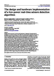
Fig. 1. Defunctionalizing Produces an Abstract State Machine. The factorial function, fac0 (left), is transformed via defunctionalization into the state machine (right). Example originally appears in Danvy [2].

Defunctionalization. Defunctionalization is a program transformation (due originally to Reynolds [38] and rejuvenated of late by Danvy et al. [1, 2]) that transforms an arbitrary higher order functional program into an equivalent abstract state machine. Defunctionalization may also be performed on monadic programs as well [2]. This section reviews defunctionalization.

(* main1 : int -> int *) fun main1 n = fac1 (n, fn a => a) (* fac1 : int*(int->int)->int *) and fac1 (0, k) = k 1 | fac1 (n, k) = fac1 (n - 1, fn v => k (n * v))

(* main2 : int -> int *) datatype cont fun main2 n = C0 = fac2 (n, C0) | C1 of int*cont (* fac2:int*cont->int *) (* appcont : cont*int->int *) and fac2 (0, k) fun appcont (C0, v) = appcont (k, 1) = v | fac2 (n, k) | appcont (C1 (n, k), v) = fac2 (n-1, C1(n,k)) = appcont (k, n * v)

Fig. 2. Defunctionalization process for the factorial function. The function, fac0 (see Fig. 1, left), is transformed into an equivalent state machine by CPS transformation (left), closure conversion (right), and defunctionalization (see Fig. 1, right).

Defunctionalizing the factorial function (Fig. 1, left) produces an equivalent state machine (Fig. 1, right). In this machine, there are three types of configurations on which the rules act; integers are initial/final configurations, pairs of type int*cont and pairs of type cont*int. The translation first performs the continuation-passing style (CPS) transformation (Fig. 2, left) to expose control flow and then performs closure conversion (Fig. 2, right) to represent the machine states as concrete, first-order data. The function fac2 resulting from closure conversion is then reformatted into the familiar arrow style for rewrite rules (Fig. 1, right). Defunctionalization for monadic programs proceeds along precisely the same lines as before once the definitions for the monadic operators (i.e., η, ?, and non-proper morphisms) are unfolded [2]. CT programs are simpler to defunc-

8

tionalize than general higher-order functions. Because the control flow within a CT program is already made manifest by its monadic structure, the CPS transformation is unnecessary. We show below in Section 5 how CT programs may be defunctionalized.

monad K = StateT (Int) G monad R = ResT K actionA actionA

:: K () = getG ?K λ g. putG (g + 1)

actionB actionB

:: K () = getG ?K λ g. putG (g − 1)

chan chan

:: Int → Int → R () = fix (λ κ. λ a. λ b. step (putG a >>K actionA >>K getG ) ?R λ newa. step (putG b >>K actionB >>K getG ) ?R λ newb. κ newa newb)

main main

:: R () = chan 0 0

Fig. 3. Example Cheap Threads program

3

Defining the Cheap Threads Language

The CT language is a proper subset of Haskell 98, extended with a special declaration form for specifying monads. It shares a concrete syntax with Haskell—in fact, any CT program may be tested in a standard Haskell environment such as GHC or Hugs, provided that Haskell definitions are supplied for the monads declared in that program. The implementation of tuples and algebraic data types, while straightforward, is not discussed in this paper in order to simplify the presentation. These features are not needed for the case study. Figure 4 gives a grammar for CT. A program consists of one or more declarations, which may be a type signature, a function declaration, a data declaration, or a monad declaration. All function declarations must be preceded by an explicit type signature. The distinguished symbol main serves as the main entry point to the program and must have type R (). An example program is given in Figure 3. The example defines two atomic state operations actionA and actionB , which respectively increment and decrement the global register G. The function

9

chan interleaves an infinite sequence of actionA operations with an infinite sequence of actionB . Between atomic operations, chan performs a context switch by saving the value of G in process A, and restoring the value of G in process B (or vice versa). As a result, the processes A and B do not affect each other’s execution, even though they both make use of the same global register. ::= decl∗ ::= tysig | fundecl | datadecl | monaddecl fundecl ::= ident ident∗ = expr datadecl ::= ∗ data dtype = condecl {| condecl} condecl ::= constr basetype∗ monaddecl ::= monad K = layer {+ layer}∗ | monad R = ResT K layer ::= StateT (basetype) ident tysig ::= ident :: type basetype ::= Int | Bool | () | (basetype{,basetype}+ ) | dtype type ::= (type) | basetype | type → type | m basetype pat ::= | ident | constr ident∗ | (ident{,ident}+ ) program decl

expr

::= | | | | | | | | | | | | | | | | | |

(expr) expr expr expr binop expr integer literal boolean literal -expr if expr then expr else expr case expr of {pat → expr}∗ (expr{,expr}+ ) () expr ?m expr expr ?m lambda expr >>m expr ηm expr fix expr fix lambda get ident put ident expr step expr

lambda ::= (lambda) | λident.expr | λident.lambda m

::= K | R

Fig. 4. Grammar for the Cheap Threads language.

While CT’s concrete syntax is borrowed from Haskell, it is fundamentally a much simpler language. We note a few important distinctions at the outset. Declaration Form for Monads. A special monad declaration form is used to construct state and resumption monads. The types and morphisms associated with these declarations are built in to the language—they are not represented in terms of the source language. We require that a program define exactly one state monad named K , and one resumption monad named R defined in terms of K . Recursion Tightly Controlled, No Mutual Recursion. Recursive functions may be defined only by explicit use of the fixed point operator fix , which only accepts tail-recursive functions. Any function not defined in terms of fix is total. Recursion without fix is not possible, because the body of a function may not refer to that function’s name, nor to any named function that does not precede it in the source text. Algebraic data types also are not allowed to be recursive. Simplified Type System. The type system dispenses entirely with polymorphism and type classes. No Higher-Order Functions. The only place where the type system allows a higher-order function to be used is as the operand to fix . Lambda expressions are only allowed to occur on the right-hand

10

side of a monadic “bind” operator, or as the operand of fix . Simplified Pattern Matching. Pattern matching is limited to deconstructing algebraic data types and tuples, and may occur only in the context of a case expression. Patterns may not be nested. Monad Declarations. CT provides built-in support for constructing monads from the standard state monad transformer StateT [28], as well as the resumption monad transformer ResT [34, 12] for concurrency. Monads are specified by a special declaration form, similar to (but less general than) that provided by MonadLab [22]. The example in Figure 5 (top) defines two monads K and R. Monad K is built from three applications of the state monad transformer, reflecting a notion of state comprised of two Int-typed registers and one Bool -typed flag. Note that StateT components must have unique names. Monad R applies the resumption transformer to K , enabling us to express interleavings of K computations.

monad K = StateT(Int) Reg1 + StateT(Int) Reg2 + StateT(Bool) Flag monad R = ResT K

getReg1 : K Int putReg1 : Int → K ()

getReg2 : K Int putReg2 : Int → K ()

getFlag : K Bool putFlag : Bool → K ()

step : K a → R a

Fig. 5. Example monad declarations in Cheap Threads (top). Non-proper morphisms produced by the declarations (bottom). N.b., step can be typed at any base type a; CT is not polymorphic.

These declarations produce “bind” and “unit” operations for the K and R monads, along with the non-proper morphisms for state and resumptions given in Figure 5 (bottom). It is important to note that these operations are primitive within the CT language; unlike their Haskell counterparts, they are not implemented in terms of newtypes, higher-order functions, etc., but instead are handled directly by the compiler. Restricting Recursion. An important design consideration of CT is that it should be implemented in a straightforward manner with loop code. To that end, one important distinction between CT and Haskell is that recursion in CT is strictly limited to tail recursive functions whose codomain is in the resumption monad. Recursive declarations must include explicit applications of the fixed point operator fix . This operator takes a function whose type is of the form

11

(τ1 → τ2 → · · · → τn → R t) → (τ1 → τ2 → · · · → τn → R t) where τ1 , τ2 , · · · , τn , t are base types (i.e. non-functional and non-monadic), and iterates it. A static check, separate from the type system, enforces the requirement that the iterated function be tail recursive. Algebraic data types also are not allowed to be recursive. Type System. CT is a simply-typed language with primitive types Int, Bool , and (); tuples and non-recursive algebraic data types; function types; and monadic types. Support for higher-order functions is limited. A simply-typed system was chosen over a polymorphic one because it makes it easier to restrict type expressiveness. Because the typing rules are mostly standard, we will discuss only the unusual cases. Due to the fact that functions are not true first-class values, partial application is not allowed, and the use of higher-order functions is limited to the built-in fix operator. These restrictions are expressed by the rule for application: Γ ` e1 , e2 , · · · , en : τ1 , τ2 , · · · , τn Γ ` f : τ1 → τ2 → · · · → τn → t (τ1 , · · · , τn , t do not contain →) Γ ` f e1 e2 · · · en : t Note that while this rule does not stop the programmer from defining higherorder functions, it does preclude the application of higher-order functions. We make this distinction rather than excise higher-order functions altogether because fix actually does operate on higher-order functions of a certain form. The monadic “bind” and “unit” operators for each supported monad are built in to the language. Rather than supply a single set of operators overloaded over all monads, the operators are subscripted to make explicit the monad in which they operate. In each of the following rules, m may stand for a monad (K or R in Figure 5 (top)), and τ , τ 0 must be base types. Γ ` ϕ : m τ Γ ` f : τ → m τ 0 Γ ` ϕ : m τ Γ ` ϕ0 : m τ 0 Γ ` ϕ ?m f : m τ 0 Γ ` ϕ >>m ϕ0 : m τ 0 Γ ` e:τ Γ ` ηm e : m τ State and resumption monad operations are also built in, and have analogous types to their Haskell counterparts [28, 34]. If the state monad K has a component StateT (τ ) Elem, it is assumed that the tags (e.g., Elem) are unique. The state operations getElem and putElem are typed as follows: Γ ` e:τ Γ ` getElem : K τ Γ ` putElem e : K () The step morphism of the R monad is typed as follows: Γ ` ϕ:K τ Γ ` step ϕ : R τ

12

Finally, the resumption monad R has an associated fixed point operator fix: Γ ` f : (τ1 → · · · → τn → R t) → (τ1 → · · · → τn → R t) Γ ` fix f : τ1 → · · · → τn → R t where τ1 , τ2 , · · · , τn , t are base types. Use of fix is subject to the further restriction (enforced by a static check outside the type system) that f is tail recursive. Notice that the argument to fix is a higher-order function. As we mentioned above, this is the only place in CT where user-defined higher-order functions may be used.

4

Compiling Cheap Threads

In this section we discuss the compilation of CT to intermediate code. The compiler targets the intermediate language described in Table 1, which we will refer to as the RTL. The RTL is a simple register transfer language. Two types of registers exist: general-purpose virtual registers (rn), and “named” registers (rs where s is a string beginning with a non-numeric character) which are used to hold global state (i.e. state components of K).

Instruction l: r := n r 1 := r 2 r 1 := r 2 + r 3

Meaning Label. Stores the constant value n in register r . Copies the value in register r 2 into register r 1. Adds the value stored in r 2 to the value stored in r 3 and stores the result in r 1. r 1 := r 2 - r 3 Subtracts the value stored in r 3 from the value stored in r 2 and stores the result in r 1. BZero r l Jumps to label l if the value stored in r is zero. Jump l Jumps to label l . Table 1. The intermediate language targeted by the compiler.

It is a simple matter to generate instructions for a RISC-like architecture from our intermediate language. We have implemented an instruction selection phase for MicroBlaze, a 32-bit RISC soft processor designed to be run on FPGA fabric. Instruction selection is entirely straightforward, so we omit the details. 4.1

Translation from Cheap Threads

This section describes the compilation of CT to the RTL. The compiler is implemented in Haskell, using the parser from the haskell-src library. Compilation proceeds in three passes: type checking (see Section 3), inlining, and code generation.

13

Inlining. In the inlining pass, all calls to non-recursive functions are inlined, starting with main at the root of the call tree. The output from the inliner is essentially one “giant term” in which the only function applications that occur are those of recursive functions, and the only variable references that occur are to λ-bound variables, which may appear only in a function passed to fix or on the right-hand side of ?m . Code Generation. After inlining, we generate code for the resulting term in a syntax-directed fashion. The code generation function codegen returns a sequence of RTL commands implementing the source expression, and the register in which those commands store the result, if any. Let CtExpr be the data type corresponding to expr in Figure 4, and RtlCom be the data type representing RTL commands. Then the type of codegen is CtExpr → CM ([RtlCom], Register ), where CM is a monad providing mechanisms for generating fresh registers and labels, and binding variables to registers. Notational Convention. For the sake of brevity, we will describe the translation rules according to the convention that peq is the code generated by translating the expression e, and anywhere after an occurrence of peq, we may refer to the register in which e’s result is stored as re . That is, peq is the list of RtlComs returned by codegen e, and re is the Register returned by codegen e. We use Haskell-style comments (beginning with a long dash — and extending to the end of a source line), and a comment at the end of the translation rule indicates which register is the result register. Compiling Pure Expressions. We first consider the compilation of pure, that is non-monadic, expressions. If the expression to be compiled is of type Int, Bool , or (), the result is simply stored in a freshly-generated register. For example, we compile addition as follows: pe1 + e2 q = pe1 q ; pe2 q ; r := re1 + re2 — Where r is fresh. Result register is r. Values of type () have no result register. Compiling Monadic Expressions. The ?m and >>m operators are compiled much like function composition. Assume without loss of generality that terms on the right-hand side of ?m are always λ-expressions. Then: pϕ ?m λx .χq = pϕq ; pχ[x 7→ rϕ ]q pϕ >>m ϕ0 q = pϕq ; pϕ0 q

— Result register is rχ . — Result register is rϕ0 .

where pχ[x 7→ rϕ ]q denotes that χ is compiled in the current environment, extended by binding variable x to register rϕ . The “unit” operator ηm serves to inject pure computations into a monad. The resumption monad operator step serves a similar function, lifting K computations into R. For step we generate a label to delineate “step-ed” state operations; for the purposes of this paper, these labels are purely informational. pηm eq

= peq

— Result register is re .

14

pstep ϕq = l : pϕq

— Where label l is fresh. Result register is rϕ .

Finally, the state monad morphisms getElem and putElem simply read or modify the associated register rElem. pgetElem q = r := rElem pputElem eq = peq ; rElem := re

— Where r is fresh. Result register is r. — No result register.

Compiling fix. As we mentioned previously, functions produced by the fix operator must be tail recursive. This means that we can compile applications of fix to simple loop code. Let f be any function satisfying this condition, with parameters named κ, v1 , v2 , · · · , vn . Call the body of this function b. p(fix f ) e1 e2 · · · en q =

pe1 q ; pe2 q ; · · · pen q l: pbq — in a special environment—see below — Where label l is fresh. Result register is rb .

Expression b is compiled in an environment where v1 , v2 , · · · , vn are bound to registers re1 , re2 , · · · , ren , and in which application of κ is compiled by the following special rule: pκ e10 · · · en0 q = pe10 q ; pe20 q ; · · · ; pen0 q re1 := re10 ; re2 := re20 ; · · · ; ren := ren0 Jump l — No result register. Note that the translation schema given above is slightly simplified in that it produces a separate loop for each (outermost) application of a recursive function, resulting in code duplication. This duplication can easily be avoided by memoizing the label at which pbq is stored. Example. Figure 6 gives the code generated for the example program in Figure 3. Each monadic operation compiles to only a handful of RTL instructions. The resulting code contains only 17 instructions, which one may reasonably expect, at an extremely conservative estimate, to translate to at most a few hundred machine language instructions on any given architecture. By comparison, ghc-6.10.1 compiling the same code produces a 650-kilobyte binary when targeting x86 on Windows with optimization enabled (disabling optimization produces a slightly larger binary). We believe that most of this code (432 kilobytes) is accounted for by the Haskell runtime system, and much of the remainder is code for various prelude and library functions. Of course, we do not claim that this comparison provides evidence that the CT compiler is “better” than GHC—obviously, GHC compiles a far more expressive source language, and therefore an increase in code size is inevitable. But the comparison does highlight a major advantage of a directly-compiled DSL over one embedded in Haskell: the code produced by Cheap Threads is several orders of magnitude smaller, making it more suitable for use in embedded systems.

15 -- Init G-save for A and B r1 := 0 r2 := 0 mainloop: l1: -- Restore G for process A rG := r1 -- Execute actionA r3 := rG r4 := 1 r5 := r3 + r4 rG := r5 r6 := rG

l2: -- Restore G for process B rG := r2 -- Execute actionB r7 := rG r8 := 1 r9 := r7 - r8 rG := r9 r10 := rG -- Save G vals for next iteration r1 := r6 r2 := r10 -- Loop Jump mainloop

Fig. 6. RTL code for the program in Figure 3

5

Synthesizing Circuits from Cheap Threads Programs

Producing a circuit from a Cheap Threads program proceeds in two steps. First, the source program is defunctionalized, producing an abstract state machine that is readily formatted in the syntax of the FSMLang DSL. The FSMLang compiler is used to produce VHDL code from which a hardware implementation on an FPGA may be synthesized. Section 5.1 defines the defunctionalization transformation for CT. Section 5.2 describes the design, syntax and implementation of FSMLang. 5.1

Defunctionalizing Cheap Threads.

This section formulates the defunctionalization transformation for CT. The resulting state machine, hStates, Rulesi, consists of a set of states, States, and a set of transformation rules, Rules, of type States → States. Defunctionalization takes place “by layer” in that terms typed in K are defunctionalized separately from those typed in R. Defunctionalizing Layered State Monads. The states and rules of the target machine arise directly from the definitions of K and the source term being transformed, respectively. Let us assume that K is a state monad of the form, K = StateT Reg1 (· · · (StateT Regn I ) · · · ). The elements of States are tuples determined by (1) the λ-bound variables within the program, (2) the states Regi within monad K , and an additional component for the value returned by the computation. Variables bound by λ are assumed without loss of generality to be unique and any fix bound variables (e.g., the “κ” in “fix(λκ. · · · )”) are not considered λ-bound. For the language defined in Section 3, the type of return values will always be one of Int, Bool , or (); let type Val = Int + Bool + (). Taking this into consideration, the elements of States of the target machine have type Reg1 × · · · ×Regn ×Var1 × · · · ×Varm ×Val . For each λ-bound variable or state in K , there is a corresponding component within the States type. Define c as the total number of components as: c = m + n. We define the update and read transitions, updx and readxi , as:

16

(x1 , · · · , x , · · · , xc , v ) 7→upd (x1 , · · · , v , · · · , xc , v ) x (x1 , . . . , xi , . . . , xc , v ) 7→readx (x1 , . . . , xi , . . . , xc , xi ) i

The updx transition sets the x “slot” to the value component while the readxi transition sets the value component to the current contents of xi . Each K term gives rise to one rule only and is derived in a syntax-directed manner. The get, put and unit operations are straightforward. Below, assume that 1 ≤ i ≤ n (i.e., puti and geti are defined only on components corresponding to K states) and let s = (x1 , . . . , xc , v ) be the input state in: K dputi ee = s 7→ (x1 , . . . , eval e s, . . . , xc , ()) K dgeti e = readxi K dηK ee = s 7→ (x1 , . . . , xc , eval e s) The unit computation, ηK e, is defunctionalized to a transition that only updates the return value state component to the value of e in the input state s, eval e s. The definition of eval is not given as it is an unremarkable expression interpreter. Note that, by construction, expression e will be of base type and will only refer to the components corresponding to λ-bound variables. The bind operations for K , ?K and >>K , are defined in terms of function composition. The transitions are total endofunctions on system configurations and, therefore, possess the standard notion of function composition. K dϕ >>K γe = K dγe ◦ K dϕe K dϕ ?K λx .γe = K dγe ◦ updx ◦ K dϕe Defunctionalizing R. This section first describes the defunctionalization of the resumption layer at a high level. Then equations formulating Rd−e are given next. Finally, the results of defunctionalizing the running example are then presented. Defunctionalizing an R computation produces a state machine whose state type includes one more component than does K ’s: PC ×Reg1 × · · · ×Regn ×Var1 × · · · ×Varm ×Val where PC = Int This additional component may be thought of as a “program counter” represented as an Int. The resulting state machine also includes multiple transitions. High-level overview. Whereas layered state adds functionality to CT languages in the form of put and get operations, the resumption layer adds control mechanisms in the form of step and fix . Roughly speaking, an R-computation is a sequence of K -computations chained together by ?R or >>R ; using only >>R for presentation purposes, an R-computation looks like: (step ϕ1 ) >>R · · · >>R (step ϕj ) Defunctionalizing each (step ϕi ) is performed by applying Kd−e to each ϕi and thereby producing a single corresponding rule, li 7→ri . Defunctionalizing >>R in

17

the above makes the control flow explicit by attaching a “program counter” (starting without loss of generality from 1) to states; this produces the set of rules: {(1, l1 )7→(2, r1 ), . . . , (j−1, lj−1 )7→(j, rj−1 )} Consider now a fixed computation, fix (λκ.λ¯x .γ). As it is tail recursive, occurrences of a recursive call, κ ¯e : R Val , will be accomplished by a rule that (1) updates the state variables corresponding to λ-bound variables x ¯ to the arguments e¯ and (2) changing the program counter component to point to the “beginning” of γ. Detailed formulation. We present the equations defining Rd−e in a Haskell-like notation, suppressing certain representation details for the sake of clarity. These equations are written in terms of a layered monad, M , containing an integer state for generating labels and an environment mapping recursively bound variables to their formal parameters. The specification of monad M is given in the MonadLab DSL [22], which allows monads to be specified simply in terms of monad transformers and hides certain technical details (e.g., order of application and lifting of operations through transformers): monad M = EnvT (Bindings) Env + StateT (Int) type Bindings = Var → [Var ] type Var = String MonadLab generates Haskell code defining the first four functions below; the last operator is defined as: counter = get >>= λi . put (i + 1) >> return i . rdEnv inEnv get put counter

:: M Bindings :: Bindings → M a → M a :: M Int :: Int → M () :: M Int

— read current bindings — resets current bindings

— gensym-like label generator

The defunctionalization, Rdee, is a computation of the transitions corresponding to e. Defunctionalizing a stepped K -computation first defunctionalizes its argument (ϕ), producing a transition, l7→r. This K -transition is converted into an R-transition by adjoining program counter components to both sides; (i, (x1 , . . . , xc , v)) is identified with (i, x1 , . . . , xc , v). The unit computation, (ηR e), is translated analogously to step: Rd−e :: CTExpr → M [Rule] Rdstep ϕe = counter >>= λi . return [(i , l ) 7→ (i +1, r )] where (l7→r) = Kdϕe RdηR ee = counter >>= λi . return [(i , l ) 7→ (i +1, r )] where (l7→r) = KdηK ee To defunctionalize a recursive expression, one first gets the next fresh label (i ) and reads the current bindings (β). In an expanded environment (β 0 ) that binds

18

the recursive variable (κ) to its formal parameters (v1 , . . . , vm ), the body (e) is defunctionalized to a list of rules (ρ). Assuming there is a unique label associated with κ, called Lκ , the transition list ρ is augmented with a transition, mkstart κ i, that serves as the “beginning of the loop”; the augmented list is returned: Rdfix (λκ.λv1 . · · · λvl .e)e = get >>= λi. rdEnv >>= λβ. (inEnv β 0 Rdee) >>= λρ. return (mkstart κ i : ρ) where β0 = β{κ:=[v1 , . . . , vl ]} mkstart κ i = (Lκ , x1 , · · · , xc , v ) 7→ (i , x1 , · · · , xc , v ) A recursive call is translated to a transition that takes an input state and moves to a state with label Lκ (defined above) and, in effect, this transition jumps to the head of the “loop”. For the sake of simplifying the presentation, the definition below only gives the case where κ has one argument (i.e., κ has type τ → Rτ 0 ); the full definition is analogous. This recursive call occurs within the body of an expression of form, fix (λκ.λx . body). In the following, assume that x is the inner λ-bound variable represented in the state configuration: Rdκee = counter >>= λi. return [(i, x1 , . . . , x, . . . , xc , v) 7→ (Lκ , x1 , . . . , eval e s, . . . , xc , v)] where s = (x1 , . . . , x, . . . , xc , v) This presentation is simplified also in that the details of looking up x in the bindings for κ are suppressed. Defining Rd−e for the bind operations: Rdγ >>R χe = Rdγe >>= λρ1 .Rdχe >>= λρ2 . return (ρ1 ++ρ2 ) Rdγ ?R λv .χe = Rdγe >>= λ[ρ1 ]. Rdχe >>= λρ2 . return (f v ρ1 : ρ2 ) where f :: Var → Rule → Rule f v ((i , s)7→(i 0 , s 0 )) = ((i , s)7→(i 0 , upd v s 0 )) Example. Returning to the running example presented in Fig. 3; the relevant portion of the channel code is: chan :: Reg1 → Reg2 → R () chan = fix ( λk. λa. λb. step (putG a >>K actionA >>K getG ) ?R λnewa. step (putG b >>K actionB >>K getG ) ?R λnewb. k newa newb ) Multiple declarations can be easily accommodated, but rather than elaborate on such details, assume that the two actions stand for particular transitions: (a, b, newa, newb, reg, val ) 7→ (a, b, newa, newb, reg+1, ()) — actionA (a, b, newa, newb, reg, val ) 7→ (a, b, newa, newb, reg−1, ()) — actionB The transitions of the state machine produced by defunctionalization are then:

19

initial_state = k (k,a,b,newa,newb,r,v) (1,a,b,newa,newb,r,v) (2,a,b,newa,newb,r,v) (3,a,b,newa,newb,r,v)

-> -> -> ->

(1,a,b,newa,newb,r,v) (2,a,b,a+1,newb,a+1,a+1) (3,a,b,newa,b-1,b-1,b-1) (k,newa,newb,newa,newb,r,v)

These transitions may be easily reformatted in FSMLang syntax: initial_state = state_k state_k -> state_1 where { } state_1 -> state_2 where { newa’