plausible hardware-based neural networks using evolution, de- velopment, and .... variables to the data packet (e.g. the membrane recovery variable in the ...
Hardware Implementation of a Bio-plausible Neuron Model for Evolution and Growth of Spiking Neural Networks on FPGA Hooman Shayani
Peter J. Bentley
Andrew M. Tyrrell
Department of Computer Science UCL, London, UK Email: h.lastname(at)cs.ucl.ac.uk
Department of Computer Science UCL, London, UK Email: p.lastname(at)cs.ucl.ac.uk
Department of Electronics University of York, York, UK Email: amt(at)ohm.york.ac.uk
Abstract— We propose a digital neuron model suitable for evolving and growing heterogeneous spiking neural networks on FPGAs by introducing a novel flexible dendrite architecture and the new PLAQIF (Piecewise-Linear Approximation of Quadratic Integrate and Fire) soma model. A network of 161 neurons and 1610 synapses was simulated, implemented, and verified on a Virtex-5 chip with 4210 times real-time speed with 1 ms resolution. The parametric flexibility of the soma model was shown through a set of experiments.
I. I NTRODUCTION The bewildering complexity of natural organisms, and their remarkable features such as fault-tolerance, immunity, robustness, parallelism, scalability, learning, and adaptation, has made them good sources of inspiration for engineers. Natureinspired paradigms such as Evolutionary Algorithms (EA), Artificial Neural Networks (ANN), and Artificial Immune Systems (AIS) are all efforts to imitate nature’s solutions to create adaptive, intelligent, and secure systems. However, natural systems simply outperform engineered systems in many aspects. The no-free-lunch theorem [1] implies that, for static and time-dependant problems, there is no algorithm that can perform better than all other algorithms on all problems. This is particularly clear in case of traditional approaches to computation, which have difficulties in solving natural problems like pattern recognition, optimization, and design. They can show an acceptable performance only on a very limited range of problems. For example, a statistical or heuristic object detection algorithm may perform very well for detecting faces in the input images but cannot be used for detecting hands or tools or distorted or incomplete faces. In contrast, natural systems perform very well on a wide set of natural problems. In other words they can adapt to different problems and new situations. This adaptation of natural systems can show itself in different forms. Scalability can be defined as the ability of a system to grow (i.e. to organize and employ more resources) in order to tackle more complicated problems or deal with (proportionally or even super-linearly) larger amount of work. Fault-tolerance can be thought as the ability of a system to cope with resource loss (by graceful degradation) and to
reorganize available resources to mitigate, or even recover, the impact of the loss. Robustness could be explained as the quality of a system to be capable of graceful degradation in case of a change (even sudden and/or unpredictable) in its operating environment, including its input. This definition implies generalization over input patterns and robustness to noise. It seems that all these intrinsic properties of natural systems emerge through intricate interactions of numerous elements on different levels. These elements could be atoms in a folding molecule, large molecules in a living cell, cells in a developing organism, neurons in a learning neural network, individuals in a swarm or replicating systems in an evolving population. All these processes can be imagined as manifestation of the same pattern at different levels, which are perceived on different time-scales. Evolution, development and learning are three major processes of this kind. Recreating such processes in artificial systems requires a huge amount of resources and computation power. The other option is to select a high level of abstraction and accept the curse of oversimplification, which usually happens in traditional approaches to evolutionary computation [2]. For example, running a bio-plausible developmental evolutionary neural network involves iterative nested cycles of evolution, development, and learning on different time scales. Evolvable hardware may enable us to exploit the computational resources at a lower level, leading to fine-grained system interactions, low-level parallelism, and a biologically more plausible approach compared to traditional evolutionary computing. This work is a step towards creating adaptable and bioplausible hardware-based neural networks using evolution, development, and learning processes. Here, we propose a digital neuron model suitable for developmental evolution of heterogeneous recurrent spiking neural networks on FPGAs (Field Programmable Gate Array) aiming at: flexibility, developmentfriendliness, high simulation and learning speeds, parallelism, and bio-plausibility, while having hardware implementation in mind. In the next section, the relevant literature is reviewed. In section III we introduce the new digital neuron model and its
architecture. The implementation of the digital neurons on a hardware platform is reported in section IV. Experiments on the neuron model and their results are reported in section V and VI. In the last section, these results are analysed and future work is discussed. II. BACKGROUND Many researchers evolved neural networks using different approaches. Yao reviewed some endeavours classifying them into evolving synaptic weights, evolving network architectures, evolving learning algorithms, and their combinations [3]. He concluded that combining evolutionary algorithms and neural networks can lead to significantly better intelligent systems. An evolutionary approach is particularly beneficial in case of Recurrent Neural Networks (RNN) since no systematic and effective approach for designing such networks for a given problem is proposed yet [3], [4]. A. Evolving RNNs Stanley and Miikkulainen devised an effective way of evolving topology and weights of increasingly complex RNNs called NEAT (Neuro-Evolution of Augmenting Topologies) [5]. It starts from a very simple topology and adds new nodes and connections by mutation, keeping track of the chronological order of innovations to allow meaningful crossovers. NEAT was successfully used in a number of complex control applications [5], [6], [7] and pattern generation [8]. Floreano et al. also used evolutionary spiking RNNs for real-time robot control [9]. B. Evolving Reservoirs Recently, with independent works of Buonomano [10], Maass (Liquid State Machine - LSM [11]), Jaeger (Echo State Network - ESN [12]) and Steil (Back-Propagation Decorrelation - BPDC [13]) a new technique, collectively known as Reservoir Computing (RC) [14], emerged, which is claimed to be capable of processing analogue continuous-time inputs and to mitigate the shortcomings of the RNN learning algorithms. This method is generally based on a recurrent network of (usually) non-linear nodes. This recurrent network, which is called reservoir (AKA liquid, dynamic filter,...) transforms the temporal dynamics of the recent input signals into a highdimensional representation. This multi-dimensional trajectory can then be used as latent state variables by a simple linear regression/classification or a feed-forward layer (know as readout map or output layer) to extract the salient information from transient states of the dynamic filter and generate stable outputs. The reservoir is traditionally a randomly generated RNN with fixed weights. Only the output layer is trained. Linear nature of the readout map dramatically decreases the computational cost and complexity of the training. Nevertheless, it has been shown that the topology, weights and the other parameters (e.g. bias, gain, threshold) of the reservoir elements can change the dynamics of the reservoir and thus affects the performance of the system [4], [15]. Therefore, a randomly generated reservoir is not optimal by definition.
Researchers tried to propose different measures and methods for generating and/or adapting reservoirs for a given problem or problem class [14]. However, there is none or very limited theoretical ground to specify which reservoir is suited for a particular problem due to the non-linearity of the system [4]. Moreover, with only one positive result, in case of intrinsic plasticity [16], the development of unsupervised techniques for effective reservoir adaptation is remained an open research question [14]. Another open question is the effect of the reservoir topology on the performance and dynamics of the system [4]. There is some evidence that hierarchical and structured topologies can significantly increase the performance [14]. Evolutionary algorithms, among other methods, were used for optimizing the performance of the reservoirs [17], [15], which led to some positive results. However, much work is still needed to evolve topologies, structures, and regularization/adaptation/learning algorithms. To make this happen, the evolutionary algorithm must be free to change the size, topology, structure, node properties, and learning algorithm of the RNN. An evolutionary system needs emergent properties such as scalability and modularity to be able to work on different hierarchical levels of reservoirs. C. Using Developmental processes Development as a combination of cell division, differentiation, and growth is believed to be one of the processes that can improve the scalability of evolution while it can also bring other emergent properties like regeneration and fault tolerance to digital systems [18]. Gordon [19], [20] showed that a developmental process can enhance the scalability of evolvable hardware as it uses an implicit mapping from genotype to phenotype. Liu et al. [21] proposed a model for developmental evolution of digital systems, which also exhibits transient fault tolerance. Bentley [22] compared human-designed, GP, and developmental evolutionary programs facing damage and showed that the developmental program can exhibit graceful degradation. Federici [23] showed that development can bring regeneration and fault tolerance to spiking neural network robot controllers. Hampton and Adami also proposed a new developmental model for evolution of robust neural networks and reviewed some other developmental neural networks [24]. Roggen et al. have a good review and classification of hardware-based developmental systems in [25]. D. Hardware-based POE systems Researchers have sought to create systems capable of evolving, developing and learning in situ to adapt themselves to a given problem and environment. These are called POE systems as they are aimed to show these capabilities in all three aspects of Phylogeny, Ontogeny and, Epigenesis of an organism. A spiking neural network on the POEtic chip [26] is an example of such systems. E. FPGA-based POE spiking neural networks The evolution of directly mapped recurrent spiking neural networks on FPGAs has been tackled by a few researchers
3 Syn. Presynaptic Inputs
(e.g. [25], [27]) using very simplified versions of the Leaky Integrate and Fire model (LIF) [28], [29]. Recently, Schrauwen et. al proposed a high-speed spiking neuron model for FPGA implementation based on the LIF model with serial arithmetic and parallel processing of the synapses utilising pipelining in a binary dendrite tree [30]. However, as yet none of these digital neuron models are quite suitable for a developmental model capable of regeneration and dendrite growth on FPGA. They are typically either constricted in terms of number of inputs per neuron or impose constraints on the patterns of connectivity and/or placement on the actual chip mostly due to implementation issues. They also do not allow heterogeneous networks with flexible parametric neurons and learning rules as important bio-plausible features.
3 4 5
Syn.
6
2 1 Cut point
Syn.
Soma
7
Axon
Ax
III. D IGITAL N EURON M ODEL
n Sy
Presynaptic Inputs
To improve the performance of evolution, the developmental Fig. 1. General architecture of the digital neuron (Syn: synapse unit). digital neuron model should be as flexible as possible, for any d constraint may impair evolvability. Evolution must be able to 3 n modify everything from network topology and dendrite strucy S 3 Syn. 4 tures to learning rules, membrane decay constants and other 4 5 5 c Syn cell parameters and processes. Evolution should be also free to 6 Syn create a suitable neuro-coding technique for each application. Syn. 6 2 Therefore, even the network activity is not guaranteed to be 2 Syn restricted as assumed in event-based simulation of spiking neural networks [30]. Thus, a time-step simulation technique 1 7 is used here. This model also needs to be relatively fast as Cut b Soma Syn Syn. 1 Syn point 7 running a POE system [26] involves iterative nested cycles A of evolution, development and learning. Such a fast parallel Axon Axon Axon Syn Soma spiking neural network on FPGA can also be used for real-time Soma applications. Design objectives of the digital neuron model can a Fig. 2. Example of the dendrite structure and its adaptability (Syn: synapse be summarised in order of importance as follows: unit). d 1) Flexibility and evolvability in terms of: d c • Development-friendliness of the dendrite model c Syn • Parametric flexibility of the soma model adds (or subtracts) its synaptic weight to the first arriving • Flexibility of the learning algorithm e the downstream packet. Therefore, the soma unit receives • Flexibility of the neural coding sum of membrane potential and post-synaptic currents in its e 2) Simulation and learning speed (parallelism) downstream input (DSI). After processing this packet, the b Soma Syn 3) bio-plausibility soma unit sends another Axon packet with the updated membrane Axon 4) Minimization of hardware area and resources on FPGA potential. Serial arithmetic is used in all the units to create Sy pipelined parallel n processing insideb each neuron, a meaning A. General Architecture that neighbouring unitsa process different bits of the same In the proposed model, each digital neuron consists of a set packet at the same time. Using this architecture has a number of synapse units and a soma unit connected in a daisy chain of collective benefits. First, a 2-way communication channel architecture shown in figure 1. The pre-synaptic input of each makes it possible to have a local synaptic plasticity mechanism synapse is connected to the axon of the pre-synaptic neuron. in each synapse leading to a higher level of parallelism. Most This architecture creates a 2-way communication channel and of the bio-plausible unsupervised learning mechanisms like allows the development of different dendrite structures as STDP and its variants involve a local learning process in demonstrated in the example of figure 2. The signal pairs each synapse. Secondly, it minimizes the number of local and that connect the units form a loop that conveys data packets global connections, which leads to a significant relaxation of (comprising a start bit and 16 data bits). The soma unit constraints imposed upon the network architecture as limited sends an upstream packet containing the current membrane routing resources is the major constraint in optimal utilization potential on its upstream output (USO). Synapse units pass of FPGA functional resources. Each unit needs only a global upstream packets unchanged but process downstream packets. clock signal to work. Other global signals can also be added If a synapse unit receives a pre-synaptic action potential it for global supervised learning mechanisms. Although other n Sy
Syn
Syn
Sy
n
n Sy
DSI USO
C. The Soma Unit (PLAQIF Model)
W 0 En
Spike Input
Control Unit
D
0 1
0
1
D
D
DSO Fig. 3.
USI
Internal architecture of the synapse unit.
architectures may bring about less pipeline latency, they need more local and global connections. For instance, a binary tree structure similar to [30] needs about double the number of local connections including the upstream links (excluding the global control signals). Third, it allows to develop any dendrite structure similar to biological dendrites. The user is free to trim (add) dendrite sub-trees at any point simply by cutting few connections and bypassing (inserting) the root unit of the sub-tree as shown by the dashed lines in figure 2. This can be implemented in FPGA using multiplexers or other routing resources (The detail is beyond the scope of this paper). This flexibility is vital for a developmental model that needs on-line growth and modification. Fourth, it maintains the regularity of the model by limiting the diversity of the module types (synapse and soma units) and connection types (dendrites, axons) to a biologically plausible bare minimum. This simplifies the place and route or dynamic reconfiguration process if a regular infrastructure of cells and connections (similar to [31]) is used. Finally, it is possible to add other variables to the data packet (e.g. the membrane recovery variable in the Izhikevich model [32]). B. The Synapse Unit The synapse unit, shown in figure 3, comprises a 1-bit adder (with carry flip-flop), a shift register containing the synaptic weight, two pipeline flip-flops, and a control unit. The upstream input (USI) is simply directed to the upstream output (USO) through a pipeline flip-flop. The control unit disables the adder and weight register when no spike has arrived by redirecting the downstream input (DSI) to the downstream output (DSO) through another pipeline flip-flop. When the control unit detects a spike, it waits for the next packet and resets the carry flip-flop of the adder when it receives the start bit. Then it enables the shift register and the adder until the whole packet is processed. A learning block can be simply inserted into the feedback loop of the weight register in order to realize a local unsupervised learning mechanism like STDP. This learning block can access the current membrane potential and the input. It is also possible to modify the synapse to create a digital DC current input unit by loading the DC current into the weight register.
Most of the hardware models are based on the Leaky Integrate and Fire (LIF) [29], [28] or simplified LIF neuron models [25], [27]. However, a Quadratic Integrate and Fire neuron model (QIF) is biologically more plausible compared to the popular LIF model as it can generate action potentials with latencies, has dynamic threshold and resting potentials and it can have two bistable states of tonic spiking and silence [33]. Here, a Piecewise-Linear Approximation of the Quadratic Integrate and Fire (PLAQIF) is proposed as a new soma model. Using this new model has a number of benefits in our context. While it is relatively inexpensive (in terms of hardware resources) to convert a serial arithmetic implementation of a LIF neuron model into a PLAQIF model (as shown later), PLAQIF model can generate a bio-plausible action potential. This is particularly important as we use the membrane voltage in the learning process. Moreover, the Behaviour of the model can be specified with a number of parameters (i.e. time constants and reset potential). These parameters can be placed in registers and look-up-tables (LUT) to be modified at run-time (e.g. by partial dynamic reconfiguration) or can be hard-wired for hardware minimization. Finally, it is easy to extend this model to a piecewise-linear approximation of Izhikevich model (with a wide range of bioplausible behaviours e.g. bursting, chattering, and resonating [32]) by adding another variable, if hardware budget permits. The dynamics of the QIF model can be described by a differential equation and reset condition of the form [29]: u˙ = a(u − ur )(u − ut ) + I
(1)
if u ≥ upeak then u ← ureset where u is membrane voltage, a is specifying the timeconstant, I is the postsynaptic input current, and the ur and ut are nominal resting and threshold voltages respectively, when I = 0. Note that in contrast with LIF models, the actual resting and threshold voltages are dynamic and they change with the input current I [33]. Applying first-order Euler method results in an equation of general form: uk+1 = uk + a(uk − ur )(uk − ut ) + Ik
(2)
if uk+1 ≥ upeak , then uk+1 ← ureset where k is the step number. The PLAQIF model is based on the serial arithmetic implementation of a LIF model, with equation uk+1 = uk + I − auk (for a < 1), with a little modification. The last term of LIF equation can be approximated using two taps: � � � � uk uk + (3) uk+1 = uk + Ik + P1 P2 | {z } | {z } Tap 1
Tap 2
where Pi = (−1)si · 2pi with pi and si being the parameters of ith tap. Each tap is computed by adding (or subtracting depending on si ) the shifted version (arithmetic shift right by pi bits) of the binary representation of uk .
y
QIF
PLAQIF x
y=V(x)
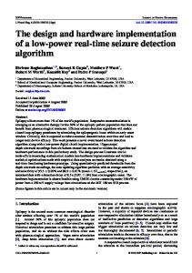
Fig. 4. The PLAQIF model approximates the QIF model (the dotted curve) with a piecewise linear function by modulating the V-shape function V (x). The three control points (with arrows) can be moved up and down by tuning the parameters.
By replacing the sign bit (S) and the most significant bit (MSB) of uk with the complement of MSB we can produce the piecewise linear function V (uk ) = |uk | − 214 (assuming a 16-bit representation). This function is shown in figure 4 as the V-shape function. By tapping (modulating) V (uk ) with different parameters (pi,0 . . . pi,3 and si,0 . . . si,3 ) for different combinations of S and MSB (positive or negative, small or large values of uk ) we get: � � � � V (uk ) V (uk ) uk+1 = uk + Ik + + (4) P1 (uk ) P2 (uk ) l x m where Pi (x) = (−1)si,j · 2pi,j , j = 14 + 1 (5) 2 It is possible to approximate eq. 2 with eq. 4 by tuning the parameters pi,j and si,j as shown in figure 4. The soma unit, showed in figure 5, comprises a 1-bit adder, a 32-bit buffer shift register (holding the partial sums from the last cycle), a 16-bit shift register (holding reset voltage ureset ), a lookup-table (LUT, a 8x5 bits RAM, which holds the parameters pi,j and si,j ), a control unit (CU, which detects the arriving packet and generates all the control signals e.g. Tap, ShiftEn, etc.), and a few multiplexers. The soma unit initiates a data packet thorough USO and waits for a packet on DSI input. At this point, the buffer holds the value uk in its left half and S and MSB flip-flops hold the sign and most significant bit of uk . The LUT selects the correct shifted version (according to S and MSB) of uk through the multiplexer and has its first bit ready on the input of the adder. The first tap starts with receiving a packet. An arriving packet, which contains the value uk + Ik goes to the other input of the adder. The LUT also selects the add or subtract operation in each tap(si ). As the operation goes on, the MSB extension block switches the jmultiplexer k to MSB at the right V (uk ) time to generate the value P1 (uk ) on the input of the j k k) adder. Therefore, the new value of uk + Ik + PV1(u (uk ) shifts into the buffer through a multiplexer. The second tap starts
immediately and the value in the left half of the buffer j goes to k k) the adder input. The other input of the adder is again PV2(u (uk ) now generated by selecting the correct shifted version of the uk from the right half of the buffer. The adder generates the updated value of u (uk+1 in eq. 4) at its output, which is shifted into the buffer and is also used to generate a new packet in the upstream output of the soma unit. This value is also used to update the S and MSB flip-flops according to the new value of uk+1 . This process continues until the peak detection block detects a transition of S without any change in MSB, which indicates an overflow, and immediately corrects the sign bit of the departing packet, generates a pulse in the axon, and initiates the absolute refractory period. The absolute refractory period, which lasts for a complete membrane update cycle, is like any other cycle except that in the second tap the output of the adder is ignored and contents of the reset voltage shift register is used instead as the new membrane potential uk+1 . The membrane update period (i.e. latency of the whole pipeline), thus neuron time constants, depend on the number of synapses n (T = 2n + 18 clock cycles). This can be compensated by the evolving parameters. IV. I MPLEMENTATION The behaviour of the neuron model was verified by VHDL simulation of a single neuron. Random spikes were fed into 16 synapses with different weights using different bio-plausible parameter settings and its membrane potential was monitored and compared to the expected dynamics of equation (4). With efficient use of the 32-bit shift registers in Virtex-5 FPGA, a random small-world network of 161 16-bit neurons with 20 inputs, 20 outputs and, 10 fixed-weight synapses per neuron, was simulated and synthesized for a XC5VLX50T chip using VHDL and Xilinx ISE tools resulting 85% utilization and a maximum clock frequency of 160MHz (i.e. pipeline throughput, which allows 4210 times faster than real-time simulation with 1 millisecond resolution). We believe that we can improve some of these figures by low-level design optimization and a cellular floor-planning similar to [31]. A single neuron and a whole network were also implemented and tested with a XC5VLX50T chip on a Xilinx ML505 development platform [34]. Through an informal verification process, timings of the neuron output spikes were checked against the simulation at the maximum clock frequency of 160 MHz using random input pulses with the same bio-plausible parameter settings use in simulation. The hardware behaviour matched the simulated model. V. E XPERIMENTS To show the parametric flexibility of the new PLAQIF soma model and to compare its behaviour and capabilities with those of biological neurons and hardware neuron models, four experiments were carried out. To explore a wide range of behaviours, arbitrary different parameter settings were selected. In the first experiment we checked if the neuron model is capable of showing both bistable and monostable behaviours of biological neurons. For bistable behaviour the ureset was
USO
DSI
D
Control Unit
MSB Tap Sign
MSB Extension
Param. LUT 4
Sub
Tap
MUX 0
0
1
1 Tap
D D
Reset Voltage
Fig. 5.
S
In the second experiment, to check the effect of changing ureset on the the F-I curve (spiking frequency against input current) of the neuron, the F-I curve was recorded using different values of the parameter ureset , keeping all other parameters fixed as follows: 4 2 214 ≤ x 3 2 0 ≤ x < 214 P1 (x) = P2 (x) = 4 14 −2 −2 ≤ x < 0 −23 x < −214 In the third experiment, the F-I curve was recorded changing the middle control point (in figure 4) keeping all other parameters fixed (ureset = −16384 and for two other control points: P1 (x) = 27 and P2 (x) = 23 when |x| ≥ 214 ). In the forth experiment, only ureset was fixed at -16384 and the F-I curves for a few different symmetric settings of pi,j and si,j (where Pi (x) = −Pi (−x), i = 1, 2) were recorded. For comparison, a QIF model of the form: I 2174 − 8000 8000 if u ≥ 30 then u ← −1
MSB
Buffer Peak Detection
Axon
Internal architecture of the soma unit
set to 17000 and for monostable behavious ureset = −16384. The other parameters were set as follows: � 7 2 0≤ x P1 (x) = −27 x