In-control performance of the joint phase II X-S control charts when ...

Quality Engineering

ISSN: 0898-2112 (Print) 1532-4222 (Online) Journal homepage: http://www.tandfonline.com/loi/lqen20

In-control performance of the joint phase II X-S control charts when parameters are estimated Lorena D. Loureiro, Eugenio K. Epprecht, S. Chakraborti & Felipe S. Jardim To cite this article: Lorena D. Loureiro, Eugenio K. Epprecht, S. Chakraborti & Felipe S. Jardim (2017): In-control performance of the joint phase II X-S control charts when parameters are estimated, Quality Engineering, DOI: 10.1080/08982112.2017.1349914 To link to this article: http://dx.doi.org/10.1080/08982112.2017.1349914

Accepted author version posted online: 20 Jul 2017.

Submit your article to this journal

Article views: 8

View related articles

View Crossmark data

Full Terms & Conditions of access and use can be found at http://www.tandfonline.com/action/journalInformation?journalCode=lqen20 Download by: [University of Alabama]

Date: 27 July 2017, At: 08:05

ACCEPTED MANUSCRIPT In-Control Performance of the Joint Phase II X -S Control Charts When Parameters Are Estimated Lorena D. Loureiro1,2, Eugenio K. Epprecht2, S. Chakraborti3, Felipe S. Jardim2

1

Fundação Oswaldo Cruz (FIOCRUZ), MS, Av. Brasil, 4365, Manguinhos, 21040-360, Rio de

Janeiro, Brazil 2

PUC-Rio, R. Marquês de São Vicente 225, 22451-900, Rio de Janeiro, Brazil

3

University of Alabama, Tuscaloosa, AL 35487, USA

Abstract The issue of the effects of parameter estimation on the in-control performance of control charts has motivated researchers for several decades. In this context, recently, acknowledging what has been called by some the practitioner-to-practitioner variability, a new perspective has been advocated, namely, the study of the conditional distribution of the in-control average run length (or the conditional false-alarm rate), which is more meaningful in practice. Adopting this new perspective, some authors have analyzed the conditional distribution of the false-alarm rate (or of the in-control average run length) of X and of S charts separately. However, since the X and

S charts are not typically used separately but together or jointly in many applications, here we study the effects of parameter estimation on the performance of the two charts applied jointly (called the joint charts). For the joint charts, defining the joint false-alarm rate as the probability that at least one of the two charts ( X and S ) issues a false alarm, we obtain its conditional distribution, some quantiles of interest (upper prediction bounds for it) and the number of Phase I

1

ACCEPTED MANUSCRIPT

ACCEPTED MANUSCRIPT samples required to guarantee that with a high probability the conditional joint false alarm rate will not exceed a maximum tolerated value. We assume normality and consider two possible estimators for the process standard deviation, as well as two possibilities regarding the X chart (1) centered at X and (2) centered at a specified target value. The results show (and we formally prove) that, whereas the required number of Phase I samples may be very large for the joint charts, interestingly, it lies between the corresponding numbers of samples required by the X chart and by the S chart individually; so, considering the performance of the charts from the perspective of their joint use may slightly alleviate the required number of Phase I samples.

Keywords: Joint X and S charts, Shewhart chart, False alarm rate, In-control average run length, Conditional and unconditional run length distribution, Conditional false alarm rate, Conditional in-control average run length, Phase I, Phase II, Parameter estimation

2

ACCEPTED MANUSCRIPT

ACCEPTED MANUSCRIPT 1. Introduction Control chart limits are based on the values of the process parameters (or, in the less frequent case of standardized control charts, these values are used to standardize the charting statistic). Typically the process parameters are not known and have to be estimated. It is well known that the use of estimated values affects the charts performance. The false-alarm rate can be larger than the nominal value (the value it would have if the process parameters where known) or, equivalently, the in-control ARL can be larger than the ARL0 value specified. There is a large bulk of research on this topic, covering the last 50 years. For literature reviews the reader is referred to Jensen et al. (2006) and Psarakis et al. (2014). With few exceptions (Trietsch and Bischak, 1998; Albers and Kalenberg, 2001, 2004; Chakraborti, 2006; Bischak and Trietsch, 2007; Gandy and Kvaløy, 2013) the works on the effect of parameter estimation on control charts performance until 2014 focused on the marginal (or ―unconditional‖) distribution of the in-control run length, on its average (the expected incontrol ARL) and sometimes also its spread (measured by its standard deviation, the unconditional in-control SDRL), and many arrived to recommendations of numbers of initial samples (Phase I samples) considered large enough to prevent the negative effect of parameter estimation (or to reduce to acceptable levels the deterioration of the charts in-control performance). These numbers of required Phase I samples are substantially larger than the classically recommended 25 or 30 samples (Montgomery, 2013), ranging (depending on the particular control chart analyzed) from 75 samples (see for example Chen, 1998, for R, S and S2 charts) to 300 samples (Maravelakis et al., 2002, for individuals charts).

3

ACCEPTED MANUSCRIPT

ACCEPTED MANUSCRIPT Recently, Saleh et al. (2015) and Epprecht et al. (2015) advocated a different viewpoint; namely, that focusing on the marginal (or unconditional) distribution of the in-control run length is inappropriate because it is an average of all possible run length distributions (rigorously: the integral, over the range of possible values of the parameters estimates — realizations of the estimators —, of the product of the run length distribution conditioned on the estimates by the pdf of the estimators) and, as a matter of fact, no actual chart’s run length will follow that distribution. (For a more detailed explanation of this point the reader is referred to Epprecht et al., 2015). Indeed, a particular chart’s actual in-control average run length (IC ARL), to take one performance measure as an example, may be much smaller than the specified ARL0 (or also much larger, depending on the errors of the estimates of the process parameters). This point had already been made by Chakraborti (2006). Saleh et al. (2015a) use the term ―practitioner-topractitioner variability‖ to refer to this effect, which the previous (unconditional) approach ignores. These works gave rise to other studies of the performance of (other types of) control charts with estimated parameters, according to the conditional approach (e.g. Saleh et al., 2015b; Aly et al., 2015 and 2016; Jardim et al., 2017). In summary, when parameters are estimated, the performance measures (ARL, false-alarm rate, run-length distribution, etc.) of any control chart are random variables, being a function of the estimators, and recent researchers focused on the properties of the conditional run-length distribution or still (in the case of Shewhart charts) on the properties of the conditional falsealarm rate distribution. With this conditional approach, they concluded that, to guarantee a desired in-control performance of the control chart, the number of initial samples required for estimating the process parameters and establishing the corresponding control limits is much

4

ACCEPTED MANUSCRIPT

ACCEPTED MANUSCRIPT larger even than the numbers previously recommended by the authors that had followed the unconditional approach. Saleh et al. (2015) studied the standard deviation of the ARL (SDARL) of X and X charts for various amounts of Phase I data and determined that the number of initial samples that makes the SDARL about 10% of the desired ARL0 was ―more than an order of magnitude larger than what previous researchers have recommended in order to have low levels of variation in the in-control ARL values among practitioners‖. Epprecht et al. (2015) studied the S chart and have calculated the number of initial samples that guarantees with a high probability (say, 0.90 or 0.95) that the conditional false-alarm rate (CFAR) of the chart would not exceed the value specified (  ) by more than a small tolerance (say, 10% or 20%). They have shown that this required number of samples could easily attain the order of several hundreds or some thousands. Jardim et al. (2017) have studied the X chart according to the same exceedance criterion and also arrived to numbers of samples of several hundreds or some thousands, even if significantly smaller than in the case of the S chart. These authors studied the X and the S charts separately; however, as it is well-known, in practice these charts are typically used together or jointly to monitor a process, as illustrated in Montgomery (2009) and emphasized, for example, in Diko et al. (2016). For the topic of joint monitoring of mean and variance, the reader is referred to the review by McCracken and Chakraborti (2013) and references therein. This motivates us to investigate the effect of parameter estimation on the performance of the joint X  S charts, and examine how this effect compares with the effect of parameter estimation on the performance of each individual chart applied separately. Thus, for example, we would like to know whether or not the number of Phase I samples required in order to guarantee a desired in-control performance of the joint X 

5

ACCEPTED MANUSCRIPT

ACCEPTED MANUSCRIPT S charts (a high probability, specified, that CFARX  S , the conditional probability that at least one of the charts issues a false-alarm, would not exceed a given tolerated value) is so large as the numbers required to guarantee the desired in-control performance of each of the two charts individually. At least it might not be so large as the larger of them. We are thus interested in the properties of the distribution of CFARX  S : its cdf, some of its quantiles that represent prediction bounds for CFARX  S (e.g. the value that is only exceeded with a probability of 0.10) and, finally, the numbers of Phase I samples required in order to guarantee with a high probability that

CFARX  S will not exceed a tolerated upper bound. The effect of parameter estimation on the performance of the joint charts was also studied by Diko et al. (2016). They analyzed the performance of classical joint X  R charts with 3-sigma limits and proposed new control charting constants to compensate for three effects: the one resulting from the implicit assumption of normality of the sample range (underlying the choice of 3-sigma limits for the S chart), the multiplicity effect (which makes the joint false-alarm rate being approximately the sum of the false-alarm rates of each of the individual charts) and the effect of parameter estimation. Our work differs from theirs in the following aspects: they focused on the X  R charts, while we here focus on X  S charts; we consider the charts with probability limits rather than 3-sigma limits (although this distinction refers only to the situation they initially consider, and disappears when they propose new charting constants that are meant to ensure the desired false-alarm rate, which make their limits also become probability limits); finally, an important difference is that they examine the performance of the charts on the basis of the unconditional in-control false-alarm rate, while we follow the conditional approach,

6

ACCEPTED MANUSCRIPT

ACCEPTED MANUSCRIPT motivated by the above mentioned considerations of practitioner-to-practitioner variability, i.e., the difference in performance between particular pairs of X  S charts that arises from the randomness of the estimators of the process parameters. We consider the charts with probability limits, each one adjusted for an intended (or ―nominal‖) individual false-alarm rate of 0.0027 (individual desired ARL0 of 370). We also consider that the quality characteristic (variable X) is normally distributed; so, for the X chart, those limits coincide with the classical ―3-sigma‖ limits. As to the S chart, unlike Diko et al. (2016) we only consider its one-sided version, without a lower control limit. While the two-sided chart is useful to detect both increases and decreases in the process standard deviation, the one-sided chart has the main objective of detecting increases in it (which correspond to process deterioration), and the use of a lower control limit would require making the upper control limit (UCL) larger, reducing the chart’s sensitivity to increases in the process dispersion. The UCL of the S chart is then based on the 0.9973-quantile of the chi-square distribution. A similar analysis could be conducted for the two-sided S chart; its lower and upper control limits would be based on the 0.00135- and the 0.99865-quantile, respectively, of the chi-square distribution. We analyze the joint performance of the joint charts in two cases: 

Case UU (―Unknown mean - Unknown variance‖): this is the most general (and typical) case, when the X chart is centered on X , the classical multiple-sample estimator of the process mean; and



Case KU (―Known mean – Unknown variance‖), when the X chart is centered on the target value. This may be justified in some applications, for example, when a machine can be adjusted for a specified process mean (nominal or target value) so that centering

7

ACCEPTED MANUSCRIPT

ACCEPTED MANUSCRIPT the chart on the nominal or target value is necessary in monitoring the process so as to detect departures from it (Montgomery, 2009). We consider that in both cases the unknown process standard deviation is estimated by S p , the square root of the the pooled variance of the Phase I samples. Mahmoud et al. (2010) have shown that the three estimators S p (biased), S p / c4 (unbiased) and c4 S p (with the smallest mean squared error), where the value of c4 to be used is for m  n  1 d.f., are more efficient than the estimator S / c4 and ―are virtually equivalent for combinations of values of m and n typically encountered in practice‖, and recommended the use of any of these three instead of the former. Although the former ( S / c4 ) is the traditional estimator of the in-control process standard deviation with S charts (see Montgomery, 2009), we see no point in using it instead of a more efficient one, given that the effort in computing one or the other is the same. Indeed, the S p estimator has been the one considered in some of the most recent papers on the effect of estimation over the performance of control charts (e.g. Faraz et al., 2015). Anyway, some results for the estimator S / c4 are available from the authors. One more point is necessary to take note of with regard to the estimation of the process variance. One might argue that, in case KU, since the in-control process mean is assumed to be known, equal to 0 , the multiple sample average of the maximum likelihood estimator

 x n

ij

j 1

 0  / n , 2

m  n  2 that is ˆ 02     xij  0  / n  / m , would be a more appropriate estimator of  02 . Indeed, i 1  j 1 

some authors (e.g. Chakraborti, 2006) have considered this estimator. We consider S p2 , even in

8

ACCEPTED MANUSCRIPT

ACCEPTED MANUSCRIPT case KU, for two reasons: first, for the sake of robustness (since in case KU the mean is not actually known; instead, the chart is meant to detect deviations from the target, which is equivalent to setting 0 equal to the target value as a specification (―mean Known‖ means indeed the in-control mean is specified); however, in Phase I the mean may not be equal to 0 in some samples, and in this case S p2 is a more robust estimator of the process variance — and S p , a more robust estimator of the process standard deviation — than the estimator based on 0 . Next, using xi to compute the i-th subgroup variance estimate is the standard procedure, reinforced by the availability of this function in statistical packages and even in ExcelTM. This estimator S p has been used, according to the same considerations, by Jardim et al. (2017), and, previously, at least by Ghosh et al. (1981). Even though the usual practice is to specify the nominal (desired) false-alarm rate (or the desired ARL0) for each chart (rather than a desired nominal joint false-alarm rate (or a joint ARL0) for the joint X  S charts), here, for the purposes of evaluation of the effect of estimation on their joint performance, we define as the nominal joint false-alarm rate, denoted by  X  S , the one the joint charts would have in the ―parameters known‖ case (Case KK), the ideal case where there is no parameter estimation. Using the independence of the statistics X and S under normality, the nominal joint false-alarm rate  X  S can be written as a function of the individual nominal false-alarm probabilities (rates)

 X and  S as (see for example, Diko et al., 2016)

 X S  1  1   X  1   S 

9

(1)

ACCEPTED MANUSCRIPT

ACCEPTED MANUSCRIPT Accordingly, we define the joint ARL0 (the nominal in-control ARL of the joint Phase II X  S charts) as the reciprocal of  X  S :

ARL0, X  S 

1

1  1   X  1   S  

.

(2)

In this paper we present results for a nominal  X S  0.0054 ( ARL0, X  S of 185), which results from Equation (1) (and Equation (2)) using the widely adopted value of 0.0027 for each of  X and  S (individual nominal IC ARL0’s of 370). Results for  X =  S = 0.005 (individual nominal IC ARL0’s of 200) and, correspondingly,  X S  0.010 , are also available from the authors. The methodology we follow for the analysis here is the same that Epprecht et al. (2015) used in the context of the S chart. The next three sections of the present paper each corresponds to a step of that methodology: in Section 2 the analytical expressions of the conditional false-alarm rate of the joint charts ( CFARX  S ) and the corresponding cdf are developed in cases KU and UU. Utilizing these cdfs, in Section 3 prediction bounds (with a low exceedance probability) are obtained for CFARX  S ; then Section 4 gives the number m of Phase I samples required in order to guarantee with a given high probability that CFARX  S will not exceed the nominal value by more than a tolerated percentage (this is done for a number of combinations of sample sizes, tolerated percentages and exceedance probabilities). An example illustrating the ideas presented in this paper is given in Section 5. Section 6 summarizes the conclusions.

2. Conditional joint false-alarm rate

10

ACCEPTED MANUSCRIPT

ACCEPTED MANUSCRIPT The control limit of the one-sided S chart (see for example Epprecht et al., 2015) for a nominal FAR of  S is

UCLS   n21,S ˆ 02 /  n  1

(3)

where n is the sample (subgroup) size in both Phase I and II, ˆ 02 is the Phase I estimator of the in-control process variance  02 and  n21, S denotes the (1–  S )-quantile of the distribution of a chi-square variable with n1 degrees of freedom. The control limits of the two-sided X chart for a nominal FAR of  X are given 

in Case KU, by:

UCLX  0  LCLX  0 



z X /2ˆ 0 (4)

n z X /2ˆ 0 n

and, in Case UU, by:

UCLX  X  LCLX  X 

z X /2ˆ 0 (5)

n z X /2ˆ 0 n

where 0 is the IC target value , X is the grand mean of the m Phase I reference samples each of size n and (as explained in Section 1) ˆ 02  S p2 is the Phase I estimator of  02 given by

11

ACCEPTED MANUSCRIPT

ACCEPTED MANUSCRIPT ˆ 02  Si2 / m where Si2    X ij  X  /  n  1 and z m

i

n

2

j

X /2

  is the 1  X 2 

  -quantile of the 

standard normal distribution. Since the control limits of the X and S charts are established as a function of the estimators of the process parameters, the signal probabilities of these charts (in particular, their false-alarm rates) are a function of those estimators. And, given that the estimators are random variables, the false-alarm rate (FAR) of each chart and the false-alarm rate of the joint charts are also random variables, conditioned on the realizations of the estimators (the estimates). It therefore makes sense to call these false-alarm rates conditional FARs (CFARs) and denote them, respectively, by

CFARX , CFARS and, for the joint charts, CFARX  S (which, one may recall, is the probability that, for any sample, at least one of the charts issues alarm when the process is in control). The notation CFAR has been employed at least by Chakraborti (2006) and Diko et al. (2016). Again, using the fact that X and S are independent under normality, as in the case of Equation (1), it can be easily shown that

CFARX S  1  1  CFARX  1  CFARS 

(6)

Let’s define the error factor of the Phase I estimate of the standard deviation as the ratio

W

ˆ 0 0

(7)

and also, in the case UU, the scaled error of the Phase I estimator of the mean as

V

0  0 . 0

(8)

In the particular case of the Phase I estimators  S p and ˆ 0  X ,

12

ACCEPTED MANUSCRIPT

ACCEPTED MANUSCRIPT W

(9)

Sp

0

and

X  0

V

0

(10) .

For the estimator S p , it is known that m  n  1W 2 follows a chi-square distribution with m  n  1 degrees of freedom (see, for instance, Chakraborti, 2007). And, the fact that





X ~ N 0 ,  02 /  mn  results, through Equation (8), in V ~ N  0, 1 /  mn   . It has been shown (Epprecht et al., 2015) that



CFARS  1  F 2 W 2  n21,S n1



(11)

where F 2 is the cdf of a chi-square variable with n1 degrees of freedom. n 1

Also, it has been shown (see, for instance, Chakraborti, 2000, 2006, 2007) that, in Case KU,



CFARX  2Φ Wz X /2



(12)

and, in Case UU (see Jardim et al., 2017),



 



CFARX  1  Φ V n  Wz X /2  Φ V n  Wz X /2   

where, Φ 

(13)

 is the standard normal cdf.

Substituting, in Equation (6), CFARS by Equation (11) and, according to the case (KU or UU),

CFARX by Equation (12) or (13), we get for the joint charts In Case KU:





CFARX  S  1   1  2Φ Wz X /2 

13

  F W n21

2

 n21,

S



(14)

ACCEPTED MANUSCRIPT

ACCEPTED MANUSCRIPT In Case UU:

CFARX  S 





 



 1   Φ V n  Wz X /2  Φ V n  Wz X /2  F 2 W 2  n21,S  n1 



 

(15)

Knowledge of the distributions of W and V enables us to calculate the cdf of CFARX  S , as we will see now. The cdf helps us understand the behavior of CFARX  S which in turn helps us better understand the in-control performance of the joint X and S charts when the parameters are estimated.

Case KU In case KU, by definition V does not come into play. Now CFARX  S can be written as g W  ,





where g W   1  1  2Φ Wz X /2

  F W n21

2

 n21,

S

  is a monotonically decreasing function

of W . Thus,





FCFARX S  b   P  g W   b   P W  g 1  b   1  FW  wb  , 0  b  1.

(16)

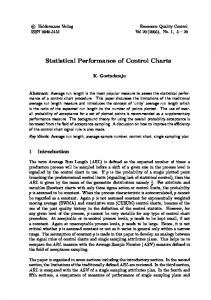
Thereby, in practice, to compute FCFARX S  b  by Equation (16), the needed wb is the particular value of W that, when substituted in Equation (14), gives CFARX S  b . Figure 1 shows 1  FCFARX S  b  (that is, the ―survival function‖, P  CFARX S  b   1  FW  wb  in Case KU using Equation (16), for sample size n  5 ,  X S  0.0054 (resulting from individual nominal ARL0’s of 370 for each chart) and several values of m (the number of initial Phase I

14

ACCEPTED MANUSCRIPT

ACCEPTED MANUSCRIPT samples).

To

this



end



FW  wb   P W  wb   P m  n  1W 2  m  n  1 wb2  F 2

m n1

note

m  n  1 wb2  where

that the

last

equality follows since, as noted before, with the estimator S p , m  n  1W 2 ~  m2  n1 . Case UU In Case UU, the CFARX  S is a function of two random variables, V and W (see Equation (15)). Hence, the cdf of CFARX  S , FCFARX S  b   P  CFARX S  b  can be obtained by integrating the joint

pdf

of

V

and

fV ,W  v, w ,

W,

over

the

region

of

the

semi-plane

{ v, w :   v  ,0  w  } that contains all pairs of points such that CFARX S  v, w  b .

Thus

FCFARX S  b   P  CFARX  S  b  

∬

 v , w:v ,0 w: CFARX S  v ,wb

fW  w  dwfV  v  dv

where we have used the fact that, since X and S 2 are independent under normality, their respective linear combinations

X

and S p2 are, also, independent, which implies the

independence of W and V , and yields fV ,W  v, w  fV  v  fW  w . To identify the region where CFARX S  v, w  b , it helps to note that, for a fixed v , CFARX  S decreases monotonically in W as in Case KU. Thus, we can write the above expression as

   b    fV  v    fW  w dw dv,  wv ,b   

FCFARX S

0  b 1

(17)

where wv , b is the particular value of W that, with V  v , yields (according to Equation (15))

CFARX S  b .

15

ACCEPTED MANUSCRIPT

ACCEPTED MANUSCRIPT As a more detailed explanation for Equation (17) note that the region of integration of the double integral that defines the cdf of CFARX  S is bounded by the curve (v, wv , b ). This is because, for any fixed v , CFARX  S is a decreasing function of W , and thus when V  v and W  wv, b , we have CFARX S  b . Therefore, the probability that CFARX S  b is the integral of the joint density of V and W over the region on the VW semi-plane { v, w :   v  ,0  w  } where W  wv, b . In other words, wv, b  w   defines the range of integration for W in the double integral that defines the cdf of CFARX  S . Now, the inner integral (inside the brackets) in Equation (17) is the survival function

1  FW  wv ,b  , so that (17) can be rewritten as FCFARX S  b  







(18)

fV  v  1  FW  wv ,b  dv

This last form is convenient for numerical computation of FCFARX S  b  since for 0  b  1 and any v  0





FW  wv,b   P W  wv ,b   P m  n  1W 2  m  n  1 wv2,b  F 2

m n1

m  n  1 wv2,b  ,

So FW  wv ,b  is the cdf of a  m2  n 1 variable (available in every statistical software including ExcelTM) at m  n  1  wv ,b  . Recall also that V ~ N  0, 1 /  mn   so it is easy to compute fV  v  2

. Still, the numerical computation is time consuming because the value of wv ,b corresponding to each value of v , although unique, cannot be determined in closed form and requires a search algorithm. Figure 2 exhibits the survival function 1  FCFARX S  b  (that is, the probability that

16

ACCEPTED MANUSCRIPT

ACCEPTED MANUSCRIPT CFARX S  b ) in Case UU, for sample size n  5 ,  X S  0.0054 (corresponding to an individual nominal ARL0 of 370 for each chart) and several values of m (the number of initial Phase I samples). Comparison of figures 1 and 2 show that the exceedance probabilities for the CFARX  S are larger in Case UU, as it might be expected because there are two parameters being estimated in contrast with Case KU where there is only one. For example, with m  25 Phase I samples, the probability that CFARX  S exceeds 0.0114 is of 20%, against 23% or 24% in Case UU. With

m  100 Phase I samples, this probability is about 4% in Case KU, against a probability of 5% in Case UU. It is interesting to note, however, that the differences between the two cases are not huge.

----- INSERT FIGURES 1 AND 2 ABOUT HERE -----

Anyway, the probability of having a CFARX  S value substantially larger than the nominal  X  S is considerable: the value of 0.0114 that has a probability of 20% of being exceeded is more than twice the nominal 0.0054, and corresponds to a conditional IC ARL of 87.7 samples. Such a short IC ARL will lead to too many false alarms. With m  100 Phase I samples, the probability that CFARX  S exceeds 0.0074 (a value 37% larger than the nominal, and which corresponds to a conditional IC ARL of 135.1 samples) is 26% in case UU and between 23 and 24% in case KU; even with 300 Phase I samples, these probabilities remain of 12% and 10 % respectively.

17

ACCEPTED MANUSCRIPT

ACCEPTED MANUSCRIPT 3. Prediction bounds Since the conditional false-alarm rate attained in an application can be much larger than the nominal false-alarm rate specified, depending on the parameter estimators, as pointed out by Epprecht et al. (2015), the user of the charts may want to know a high-probability upper bound for it, i.e., a CFAR value that presents only a (specified) low probability of being exceeded. We here follow the same path as in that paper, now for the joint X  S charts. In formal notation, for given m and n, the user may want to know the value c such that P  CFARX S  c   p

where 0  p  1 is small — for example, 0.05 or 0.10. So, c is the (1p)-quantile of CFARX  S : 1 c  FCFAR 1  p  X S

These bounds can be obtained from Equations (15) and (14) as explained below. In Case KU, since CFARX  S is a monotonically decreasing function of W (see Equation (14)), the (1p)-quantile of CFARX  S is the value of this function at the p-quantile of W:



1 FCFAR 1  p   CFARX S FW1  p  X S



(19)

Thus, the prediction bound of probability (1p) for CFARX  S can be determined by substituting FW1  p  for W in Equation (14). The knowledge of the distribution of W, or rather, of

m  n  1W 2 , which is a chi-square with m  n  1 df, makes this determination easier.

On the other hand, in Case UU, the fact that CFARX  S is a function of two random variables renders the calculation of the prediction bounds by a direct formula like Equation (19) rather

18

ACCEPTED MANUSCRIPT

ACCEPTED MANUSCRIPT intractable. In this case, we obtained the prediction bounds by direct search: we used the same approach indicated in Section 2 for determining FCFARX S  b   P  CFARX S  b  , now varying b in an univariate search to find the value that gave the desired value for the cdf. The 0.90 and 0.95 quantiles of CFARX  S determined for a joint  X  S of 0.0054 (resulting from individual  X and  S nominal values of 0.0027) and some combinations of sample size (n) and number of Phase I samples (m) are given in Table 1. These quantiles are upper prediction bounds for CFARX  S : values of CFARX  S that have only a small probability (namely 5% and 10%) of being exceeded. ----- INSERT TABLE 1 ABOUT HERE -----

To see how larger CFARX  S can be from the nominal joint false-alarm rate, with a nonnegligible probability, it is enough to look at Table 1. Inspection of this table reveals that, with sample sizes up to n = 10, the usual recommendations of m  25 Phase I samples lead to a 10% probability that CFARX  S is by far larger than the nominal value of 0.0054. With n = 5, the 10% probability is that it is more than 200% larger than nominal, and even with n = 20 or 25, the 10% probability is that it is more than 100% larger. This means that IC ARLs have a probability of 10% of being, respectively, less than 3 or 2 times smaller than the nominal value of 185. Even with 100 Phase I samples of size up to n = 10, there is a probability of 10% that CFARX  S exceeds the value of 0.0054 by more than 50% (with n = 5, the 10% probability is that CFARX  S exceeds 0.0054 by more than 74% in Case KU and by more than 78% in Case UU).

19

ACCEPTED MANUSCRIPT

ACCEPTED MANUSCRIPT Even with 300 Phase I samples, with sample sizes up to n = 10, there is a 10% probability that

CFARX  S is more than 30% larger than nominal; with n = 5, even with 1000 Phase I samples, there is a 10% probability that CFARX  S is more than 20% larger than nominal. The prediction bounds (upper quantiles) of CFARX  S do not differ much between cases UU and KU, except for the smaller numbers of Phase I samples (25 and 50). These findings are similar to the ones obtained by Epprecht et al. (2015) regarding the S chart, and by Saleh et al. (2015) regarding the X chart; namely, that even with hundreds of Phase I samples there is a non-negligible chance that the IC performance of the charts is significantly worse than the nominal. Analyzing the charts separately, in percent terms, the deterioration (relative to the nominal false-alarm rate) is larger with the S chart (with  X  0.0027) than with the X chart (with  S  0.0027); the deterioration of CFARX  S (with  X  S  0.0054) lies in between. A formal proof of this fact is given in Appendix A. To give a quantitative idea of this effect, Table 2 gives the ratios of the CFAR prediction bounds to the nominal false-alarm rates of the joint X  S charts and of the X and the S charts individually, for  X  S  0.0054 and  X   S  0.0027. The prediction bounds for the X chart (needed for computing the ratios) are given in Jardim et al. (2017) and the prediction bounds for the S chart were calculated by us as in Epprecht et al. (2015), for  S  0.0027 (since the prediction bounds given in that paper are for  S  0.0050).

20

ACCEPTED MANUSCRIPT

ACCEPTED MANUSCRIPT

----- INSERT TABLE 2 ABOUT HERE -----

4. Required number of Phase I samples for guaranteed IC performance

The prediction bounds in Table 1 indicate if a given number of Phase I samples is sufficient to guarantee a desired in-control performance of the joint charts in Phase II, but these limits are here given only for the specific numbers of samples in the tables (25, 50, 100, 300 and 1000). The final user of the charts may want to know what is the number m of Phase I samples required in order to guarantee with a given high probability 1  p that CFARX  S will not exceed the nominal value by more than a tolerated percentage 100 , that is, what is the minimum m such that P CFARX S  1     X S   p , or FCFARX S 1     X S   1  p . It is not possible to obtain m directly; we obtained it by search, for given values of n,  , p and

 X  S . The Case KU is easier since for each tuple (n,  ,  X  S ) the ( 1  p )-quantile of CFARX S is obtained by substituting the p-quantile of W in Equation (14), but a search is still required because Equation (14) cannot be solved analytically. In Case UU, the search is much more timeconsuming, involving repeated evaluation of Equation (18). Tables 3 and 4 give the values of m for some combinations of  and p, for  X  S = 0.0054 and for some values of n.

----- INSERT TABLES 3 AND 4 ABOUT HERE -----

21

ACCEPTED MANUSCRIPT

ACCEPTED MANUSCRIPT

Inspection of tables 3 and 4 reveals that the required number of Phase I samples (m) varies substantially with n,  and p, decreasing with the increase of any of these factors. In the range of values of n,  and p considered, m varies from about 5500 down to 50 samples. Considering a shorter range for these factors, namely n  5, 10 ,  0.10, 0.20 and p 0.05, 0.10 , m still varies from about 5500 down to less than 600 samples. The differences in m according to the case, KU or UU, (for same values n,  and p) are small nevertheless. The differences increase with n,  and p, but remain of less than 10% in the worst cases. As a consequence of the larger spread of the pdf of the CFAR of the S chart relative to the pdf of the CFAR of the X chart (either in the KU or in Case UU), which makes the prediction bounds of the joint X  S charts lie between the ones of the X chart and of the S chart alone (as seen in the previous section), a similar effect is observed with the minimum number m of Phase I samples that guarantee with probability 1  p that CFAR will not exceed the nominal value by more than a tolerated percentage 100 : for equal values of  and p, and of course for the same sample size n, we have that mX  mX S  mS , where the subscripts indicate the chart being considered (or the joint charts, in the case of the subscript X  S ). For a formal proof of this effect, see Appendix B. For a quantitative appreciation of this effect, Table 5 gives, for some values of  , p and n (considering  X  S  0.0054 and individual  X and  S values of 0.0027), the values of mX and mS and, for facility, repeats the corresponding values of mX  S from Tables 3 and 4. The values of mX were given in Jardim et al. (2017); the values of mS have been

22

ACCEPTED MANUSCRIPT

ACCEPTED MANUSCRIPT calculated by us for the nominal  S of 0.0027 because the values available in Epprecht et al. (2015) are for  S  0.0050. The table confirms that the values of mX  S are larger than the values of mX , but smaller than the values of mS , for same n,  , p. This means that the severity of the effect of estimation on the IC performance of the joint charts in Phase II is between the severities of the effect in the cases of the X chart and of the S chart individually. As a result, considering the performance of the charts jointly slightly alleviates the requirement of large number of Phase I samples, although these numbers still remain very large. ----- INSERT TABLE 5 ABOUT HERE -----

5. Example We illustrate the ideas by applying the joint X  S charts in a semiconductor manufacturing process. A more detailed description of this example and the data are given in Montgomery (2009, p. 183). Semiconductors are heavily used in all modern electronic devices such as computers and smartphones. An important step in semiconductor fabrication is photolithography, which has a sub-step called ―hard-bake‖ process to increase the adherence and the etch resistance of a light-sensitive photoresist material. The hard-bake process introduces some stress into the photoresist and as a result some shrinkage or expansion may occur. Thus, an important quality variable to be monitored is the measure of how much the photoresist shrinks or expands due to the baking process, i.e., the flow width of the photoresist. In this example, the flow width follows a normal distribution with an in-control mean ( 0 ) of 1.5 microns and an incontrol standard deviation (  0 ) of 0.15 microns. However, usually these parameters are

23

ACCEPTED MANUSCRIPT

ACCEPTED MANUSCRIPT unknown and must be estimated. Twenty-five Phase I reference samples ( m  25 ), each of size five ( n  5 ) of the flow width measurements are provided in Montgomery (2009, p. 232). These are used to estimate 0 and  0 (Case UU) and subsequently calculate the control limits of the joint X and S charts. For each individual chart, a nominal false-alarm rate of 0.0027 (i.e.,

 X  0.0027 and  S  0.0027 ) is used; hence, according to Equation (1), the joint nominal false-alarm rate (  X  S ) is 0.0054. However, at the outset, before starting parameter estimation and control limits calculation, note that there may be an issue with the available amount of data. For example, from Figure 2, it is seen that the joint conditional false-alarm rate ( CFARX  S ), has a large variability (see the different curves); the variability is the highest when m  25 (the solid curve), and decreases with increasing m (see the other curves) being the lowest when m  1,000 . The large variability is a problem. Take for example the point (0.0124, 0.20) in the solid curve (

m  25 ), which indicates that there is a 20% probability that the CFARX  S exceeds 0.0124, a value 2.3 times larger than the nominal value of 0.0054, and that would result in an in-control ARL of only 80.6. This is obviously undesirable, but note that the variability and so the high quantiles of CFARX  S decrease with increasing m , which makes the case for larger m values. In fact, using the reference data at hand, we find, for ˆ 0 , X  1.5056 and, for ˆ 0 , S p  0.1391 so that the error factor V  0.0373 [see Equation (7)] and the scaled error W  0.9273 [see Equation (8)], which yield, using Equation (15), CFARX S  0.0129. This value is more than two times larger than the nominal value of 0.0054, and is of course problematic in that there will be many more false alarms than nominally expected. This illustrates the possible impact of

24

ACCEPTED MANUSCRIPT

ACCEPTED MANUSCRIPT parameter estimation in actual applications of the joint X  S charts. Also, from Figure 2, it can be seen that the actual and undesirable value of 0.0129 is not very unlikely, since the probability that CFARX  S exceeds 0.0129 is close to 20%. This is where the prediction bounds calculated and reported in Table 1 are useful: they represent the values of c for a given m and n so that the probability that CFARX  S exceeds c is 10 (or 5) percent, as specified by the user. For example, for m  25 and n  5, the probability that CFARX  S exceeds 0.0172 is 5%. But 0.0172 is much larger than the nominal 0.0054 and even larger than the actual 0.0129 , and thus is practically undesirable. So, the conclusion from this analysis is that the amount of reference data used in this example for parameter estimation and subsequent construction of Phase II control limits is simply not enough to guarantee a satisfactory in-control performance of the joint X  S charts in Phase II.

The natural follow-up question for the practitioner then is the minimum amount of Phase I data that guarantees with a high probability (say 90% or 95%) that CFARX  S does not exceed the nominal false alarm rate by more than a specified small tolerated percentage (e.g. 20%). This information can be found from Table 3. For example, given a sample size of five (

n  5 ), in order to guarantee that P CFARX S  1.2  0.0054 = 10%, a minimum of m  909 samples are necessary, i.e., a total of 4,545 flow width measurements. To further examine the impact of parameter estimation of the joint X  S charts in Phase II operations we calculate the control limits according to Equations (3) and (5) and the reference data, obtaining UCLS  0.2665 , UCLX  1.692 and LCLX  1.3190. Next we simulate a series of independent Phase II samples, each of size 5, from the in-control distribution of the flow

25

ACCEPTED MANUSCRIPT

ACCEPTED MANUSCRIPT width (of the hard-bake process) which is assumed to be a normal distribution with mean

0  1.5 and standard deviation  0  0.15 . We also calculate the sample mean and standard deviation for each simulated sample and plot these on the respective control chart with the control limits. The joint charts are shown in Figure 3. As it can be seen, the first signal occurs on the X chart, on the 138th sample, so the in-control run length is 113. With the signal, the user would typically suspect that an assignable cause has occurred at or before that time. But, since we simulated in-control data, this is a false alarm. This false alarm occurred much earlier than what is nominally expected, which would be around the 185th sample (1/0.0054 = 185.19). This again illustrates the deleterious effects of parameter estimation on the joint X and S control charts which is better understood through an examination of the conditional run length distribution and its attributes such as the conditional false-alarm rate (or the conditional incontrol average run length).

----- INSERT FIGURE 3 ABOUT HERE -----

6. Conclusions We analyze the effect of parameter estimation on the in-control performance of the Phase II joint X  S charts, obtaining analytical expressions for the joint conditional false-alarm rate (

CFARX  S ), i.e., the probability that, at any given sample, at least one of the two charts issues a false alarm, in two cases: when both the mean and standard deviation of the process are unknown and need to be estimated (case UU), and when only the standard deviation is estimated (case KU;

26

ACCEPTED MANUSCRIPT

ACCEPTED MANUSCRIPT IC mean specified/known). Tables are given for the upper quantiles of CFARX  S distribution, which constitute prediction bounds for the actual false-alarm rate a particular pair of charts has in a given application. Also, we provide the number of Phase I samples required in order to guarantee a specified in-control performance, in terms of keeping the probability that CFARX  S exceeds a (specified) tolerated value limited to a small (specified) value. We consider the charts with probability limits, each with a nominal in-control ARL of 370, using S p (the square root of the pooled variance) to be the estimator of the process standard deviation. Results for a nominal in-control ARL of 200 (for each chart) and for the estimator S / c4 are available upon request. Note that we considered the one-sided S chart without an upper control limit. It has been seen in Section 4 that the numbers of Phase I samples required to guarantee the desired performance of the chart are larger for the S chart than for the X chart, given the same conditions (namely, the same probability p that the conditional false-alarm rate exceeds the nominal value by the same percentage). It is interesting to note that the numbers of Phase I samples required to guarantee the desired joint in-control performance of the X  S charts in Phase II (under the same conditions and considering as the nominal false-alarm rate of the joint charts the probability that at least one of them issues a false alarm when each individual chart’s false-alarm probability equals the nominal false-alarm rate) are between the numbers of samples required for the X chart and for the S chart. As a concrete example: to an individual false-alarm rate of 0.0027 for each individual chart corresponds a joint false-alarm rate of 0.0054 for the joint charts; the number of Phase I samples required to ensure, with a probability of 0.90, that the actual joint false-alarm rate does not exceed 0.0054 by more than 20% lies between the number

27

ACCEPTED MANUSCRIPT

ACCEPTED MANUSCRIPT of Phase I samples required to ensure with a probability of 0.90 that the actual false-alarm rate of the X chart does not exceed 0.0027 by more than 20% and the number of Phase I samples required to ensure with a probability of 0.90 that the actual false-alarm rate of the S chart do not exceed 0.0027 by more than 20%. In summary, the number of Phase I samples that guarantees a desired IC performance (i.e., that limits, with a high probability, the false-alarm rate to a tolerated bound) for the pair of charts as a whole is between the number of Phase I samples required to guarantee the desired IC performance for each chart individually. Nevertheless, the required number of Phase I samples is still very large for practical purposes. This motivates the investigation of adjustments to the control limits of the joint X  S charts (studied, for the S chart alone, by Faraz et al., 2015, and also by Goedhard et al., 2017b; and, for the X chart alone, by Goedhard et al., 2017a, and by Jardim et al., 2017) from the perspective of their joint performance. This will be the subject of a future paper.

Acknowledgements This research was partly supported by the CNPq (Brazilian Council for Scientific and Technological Development) through projects numbers 308677/2015-3 (2nd author), 401523/2014-4 (3rd author) and 201172/2016-0 (4th author) as well as by CAPES (Brazilian Coordination for the Improvement of Higher Education Personnel) through a national PhD scholarship for the 4th author. We are also grateful to two anonymous reviewers for their feedback and to the Editor, whose suggestions improved the quality of the paper. Authors’ Bio

28

ACCEPTED MANUSCRIPT

ACCEPTED MANUSCRIPT

Lorena Drumond Loureiro holds MSc and PhD degrees in Industrial Engineering by PUC-Rio and works in Fundação Oswaldo Cruz (FIOCRUZ), a foundation responsible for health surveillance in Brazil. This is her second paper on the subject of the effect of parameter estimation on control charts from the conditional performance perspective. Eugenio Kahn Epprecht is an Associate Professor at the Dept of Industrial Engineering of PUC-Rio. His major research interest is Statistical Process Control. He has published articles in journals such as C&OR, IIE Transactions, IJPE, IJPR, JAS, The Journal of Chemometrics, JQT, QE, QREI, QTQM, among others. He has been a member of the ISBIS (International Society for Business and Industrial Statistics) council, and has organized the 2nd International Symposium on Statistical Process Control (ISSPC’2011). He is a member of ASQ. Subhabrata (Subha) Chakraborti holds a PhD in Statistics by the State University of New York; he is Professor of Statistics, Robert C. and Rosa P. Morrow Faculty Excellence Fellow, Fellow of the American Statistical Association, an Elected member of the International Statistical Institute and a Fulbright Senior Scholar to South Africa. His specialty areas are Nonparametric and Robust Statistical Inference with applications in areas such as Statistical Process Control, Survival/Reliability Analysis, Econometrics, Statistical Computing, and Extreme Values. He has over one hundred publications in a variety of outlets, including national and international peer-review journals and is a co-author of the book Nonparametric Statistical Inference, fifth edition, published by Marcel Dekker. He has been a visiting professor at a great number of universities abroad, in India, Brazil, France, South Africa and Turkey and has won a number of teaching and research excellence awards. He has served as an Associate Editor of

29

ACCEPTED MANUSCRIPT

ACCEPTED MANUSCRIPT Communications in Statistics for over fifteen years. He is a member of the American Statistical Association and the International Statistical Institute. Felipe Schoemer Jardim holds an BSc degree in Electrical Engineering (Decision Support Systems) by PUC-Rio and an MSc degree in Industrial Engineering also in PUC-Rio, where he is currently a doctoral student. He spent a research visit to the University of Alabama, USA and presented a paper at the 2016 Joint Statistical Meetings in Chicago. His current research interests are in Statistical Process Control with an emphasis on the effects of parameter estimation on control chart performance.

30

ACCEPTED MANUSCRIPT

ACCEPTED MANUSCRIPT References ALBERS, W. and KALLENBERG, W. C. M. (2004). Are Estimated Control Charts in Control? Statistics 38(1): 67-79. ALBERS, W. and KALLENBERG, W. C. M. (2004). Estimation in Shewhart control charts: effects and corrections. Metrika 59(3): 207–234. ALY, A. A.; MAHMOUD, M. A.; and WOODALL, W. H. (2015). A comparison of the performance of phase II simple linear profile control charts when parameters are estimated. Communications in Statistics - Simulation and Computation, 44(6): 1432-1440. ALY, A. A.; MAHMOUD, M. A.; and HAMED, R. (2016). The performance of the multivariate adaptive exponentially weighted moving average control chart with estimated parameters. Quality and Reliability Engineering International, 32(3): 957-967. BISCHAK, D. P. and TRIETSCH, D. (2007). The Rate of False Signals in X Control Charts with Estimated Limits. Journal of Quality Technology 39(1): 54 - 65. CHAKRABORTI, S. (2000). Run Length, Average Run Length and False Alarm Rate of Shewhart X-bar Chart: Exact Derivations by Conditioning. Communication in Statistics Simulation and Computation 29(1): 61-81. CHAKRABORTI, S. (2006). Parameter Estimation and Design Considerations in Prospective Applications of the X Chart. Journal of Applied Statistics 33(4): 439–459. CHAKRABORTI, S. (2007). Run Length Distribution and Percentiles: The Shewhart X Chart with Unknown Parameters. Quality Engineering 19: 119–127.

31

ACCEPTED MANUSCRIPT

ACCEPTED MANUSCRIPT DIKO, M. D., CHAKRABORTI, S. and GRAHAM, M. A. (2016). Monitoring the Process Mean When Standards Are Unknown: A Classic Problem Revisited. Quality and Reliability Engineering International 32(2): 609-622. EPPRECHT, E. K., LOUREIRO, L. D. and CHAKRABORTI, S. (2015). Effect of the Amount of Phase I Data on the Phase II Performance of S2 and S Control Charts. Journal of Quality Technology 47(2): 139-155. FARAZ, A., WOODALL, W. H., & HEUCHENNE, C. (2015). Guaranteed conditional performance of the S2 control chart with estimated parameters. International Journal of Production Research 53(14): 4405-4413. GANDY, A. and KVALØY, J. T. (2013). Guaranteed Conditional Performance of Control Charts via Bootstrap Methods. Scandinavian Journal of Statistics 40: 647-668. GOEDHART, R., SCHOONHOVEN, M. and DOES, R. J. M. M. (2017a). Guaranteed InControl Performance for the Shewhart X and X Control Charts. Journal of Quality Technology 49(2): 155-171. GOEDHART,

R.,

SILVA,

M.

M.,

SCHOONHOVEN,

M.,

EPPRECHT,

E.

K.,

CHAKRABORTI, S., DOES, R. J. M. M. and VEIGA FILHO, A. L. (2017b). Shewhart Control Charts for Dispersion Adjusted for Parameter Estimation. IISE Transactions, 2017, accepted.. JARDIM, F. S., CHAKRABORTI, S. and EPPRECHT, E. K. (2017) Effect of the Amount of Phase I Data on the Conditional Performance of the Phase II X Chart. Technical Memorandum 01/2017, Department of Industrial Engineering, PUC-Rio.-

32

ACCEPTED MANUSCRIPT

ACCEPTED MANUSCRIPT JENSEN, W. A.; JONES-FARMER, L. A.; CHAMP, C. W.; and WOODALL, W. H. (2006) Effects of Parameter Estimation on Control Chart Properties: A Literature Review. Journal of Quality Technology 38(4): 349-364. MAHMOUD, M. A.; HENDERSON, G. R.; EPPRECHT, E. K.; and WOODALL, W. H. (2010) Estimating the Standard Deviation in Quality Control Applications. Journal of Quality Technology, 42(4): 348-357. MCCRACKEN, A. K. AND CHAKRABORTI, S. (2013). Control Charts for Joint Monitoring of Mean and Variance: An Overview. Quality Technology & Quantitative Management, 10(1): 17-36. MARAVELAKIS, P. E.; PANARETOS, J.; AND PSARAKIS, S. (2002). Effect of Estimation of the Process Parameters on the Control Limits of the Univariate Control Charts for Process Dispersion. Communication in Statistics—Simulation and Computation 31(3): 443–461. MONTGOMERY, D. C. Statistical Quality Control: A Modern Introduction (7th ed.). John Wiley & Sons, Singapore Pty. Ltd, New York, 2013. MONTGOMERY, D. C. Statistical Quality Control: A Modern Introduction (6th ed.). John Wiley & Sons, Singapore Pty. Ltd, New York, 2009. PSARAKIS, S.; VYNIOU, A. K.; and CASTAGLIOLA, P. (2014). Some recent developments on the effects of parameter estimation on control charts. Quality and Reliability Engineering International, 30(8): 1113-1129. SALEH, N. A.; MAHMOUD, M. A.; KEEFE, M. J.; and WOODALL, W. H. (2015a) The Difficulty in Designing Shewhart X and X Control Charts with Estimated Parameters. Journal of Quality Technology 47(2): pp.127-138

33

ACCEPTED MANUSCRIPT

ACCEPTED MANUSCRIPT SALEH, N. A.; MAHMOUD, JONES-FARMER, L. A.; ZWETSLOOT, I. and WOODALL, W. H. (2015b) Another Look at the EWMA Control Chart with Estimated Parameters. Journal of Quality Technology 47(4): pp.363-382. TRIETSCH, D. and BISCHAK, D. (1998) The Rate of False Signals for Control Charts with Limits Estimated from Small Samples . In: Proceedings of the 33rd Annual Conference, The Operational Research Society of New Zealand, 232-241.

34

ACCEPTED MANUSCRIPT

ACCEPTED MANUSCRIPT

Appendix A Proof that the deterioration of the performance of the joint charts due to parameter estimation lies proportionally between the deteriorations of the performances of each chart:

Equation (1) can be rewritten as

 X S   X   S   X  S Similarly, Equation (6) can be rewritten as

CFARX S  CFARX  CFARS  CFARX CFARS Consider the CFAR’s that correspond to a given upper percentile (e.g. 90%) of their respective distributions, i.e., prediction bounds

1 FCFAR 1  p  ; let’s represent the deterioration in

performance of the charts by the ratios k X , k S and k X  S of these bounds to the respective nominal FAR’s (  X ,  S or  X  S ). Then CFARX  k X  X , CFARS  kS S and the ratio between

CFARX  S and  X  S is k X S 

CFARX  S

 X S



k X  X  kS S  k X k S X  S  X  S  XS

Given that  X and  S are substantially smaller than the unity, the term  X  S in the denominator is negligible (some orders of magnitude smaller than  X and  S ). The same is true about the term k X kS X  S in the numerator, even if k X and k S are larger than the unity (but not by orders of magnitude). As a result, the ratio between the prediction bound of CFARX  S and the nominal FAR of the joint charts is approximately

35

ACCEPTED MANUSCRIPT

ACCEPTED MANUSCRIPT k X S 

 X k X   S kS  X  S

which is a weighted average of k X and k S . Most typically,  X   S   and k X  S becomes simply the average  k X  kS  / 2 . Appendix B Proof that the number of Phase I samples that guarantees that, for the joint charts,

P CFARX S  1     X S   p lies between the number of Phase I samples that guarantees that, for the X chart, P CFARX  1     X   p and the number of Phase I samples that guarantees that, for the S chart, P CFARS  1     S   p :

In Appendix A it was proven that, with equal sample size n and equal number of Phase I samples, m, the ratio k X  S 

CFARX  S

 X S

of the prediction bounds for a given percentile of

CFARX  S to the nominal joint false-alarm rate  X  S lies between the similar ratios kX 

CFARX

X

and kS 

CFARS

S

, of the prediction bounds of the X and of the S chart to their

nominal false-alarm rates. This holds in general and also, in particular, for CFAR values that are particular p-quantiles of the CFAR distributions (i.e., prediction bounds with probability 1  p ). Let’s write each of the ―k’s” as 1    where, now, 100 represents the 1  p  -probability prediction bound of the percent increase in the false-alarm rate CFAR (rather than a tolerated percent increase) with respect to the nominal value  . In other words, let’s write

36

ACCEPTED MANUSCRIPT

ACCEPTED MANUSCRIPT k X S  1   X S , k X  1   X and kS  1   S . Then the fact that k X  S lies between k X and k S implies that, with the same n, m (let’s denote this value of m by m0) and p,  X  S lies between  X and  S . Let’s consider that  X   S ; so, with a same number m0 of Phase I samples,  X   X S   S . (If the order were the inverse of that, the same argument would apply, just symmetrically). This means that the number of samples that limits to p the probability that CFARX exceeds  X by more than 100  X  S % is smaller than m0 and the number of samples that limits to p the probability that CFARS exceeds  S by more than 100  X  S % is larger than m0. In other words, the number of Phase I samples that limits to a given value p the probability that the joint CFAR exceeds the nominal joint false-alarm rate by more than a tolerated percentage 100 lies between the numbers of samples required for limiting to the same value p the probabilities that the individual CFARs of the X chart and of the S chart, separately, exceed their respective nominal false-alarm rates by the same percentage 100 .

37

ACCEPTED MANUSCRIPT

ACCEPTED MANUSCRIPT

𝑷(𝑪𝑭𝑨𝑹𝑿̅

𝑺

P(CFARJ>b); n = 5; αJ= 0.0054

𝒃)

m = 25

0,55

m = 50

0,50

m = 100

0,45

m = 300

0,40

m = 1000

0,35 0,30 0,25 0,20 0,15 0,10 0,05

Figure 1:

̅

c.d.f. complement, (

38

̅

0,0304

0,0294

0,0284

0,0274

0,0264

0,0254

0,0244

0,0234

0,0224

0,0214

0,0204

0,0194

b

0,0184

0,0174

0,0164

0,0154

0,0144

0,0134

0,0124

0,0114

0,0104

0,0094

0,0084

0,0074

0,0064

0,00

0,0054

P(CFARJ>b)

0,60

) – Case KU,

ACCEPTED MANUSCRIPT

ACCEPTED MANUSCRIPT

𝑷(𝑪𝑭𝑨𝑹𝑿̅

𝑺

P(CFARJ >b), n = 5, αJ = 0.0054

𝒃)

0,60

m=25 0,55

m=50

0,50

m=100 m=300

0,45

m=1000

0,35 0,30 0,25 0,20 0,15 0,10 0,05

0,0304

0,0294

0,0284

0,0274

0,0264

0,0254

0,0244

0,0234

0,0224

0,0214

0,0204

0,0194

0,0184

0,0174

0,0164

0,0154

0,0144

0,0134

0,0124

0,0114

0,0104

0,0094

0,0084

0,0074

0,0064

0,00

0,0054

P(CFARJ >b)

0,40

b

Figure 2:

̅

c.d.f. complement, (

39

̅

) – Case UU,

ACCEPTED MANUSCRIPT

ACCEPTED MANUSCRIPT Xbar chart

1.800 1.700

Phase I

Phase II

1.692

1.600 1.506

1.500 1.400 1.319 1.300 1.200 1 4 7 10 13 16 19 22 25 28 31 34 37 40 43 46 49 52 55 58 61 64 67 70 73 76 79 82 85 88 91 94 97 100103106109112115118121124127130133136

S chart 0.3 0.2665

Phase I

Phase II

0.25

0.2 0.15 0.1

0.05 0 1 4 7 10 13 16 19 22 25 28 31 34 37 40 43 46 49 52 55 58 61 64 67 70 73 76 79 82 85 88 91 94 97 100103106109112115118121124127130133136

Figure 3: The Phase 1 and Phase 2 of the ̅  charts in the Hard-Bake Process

40

ACCEPTED MANUSCRIPT

ACCEPTED MANUSCRIPT

Table 1: 90% and 95% prediction bounds for 90th percentiles



Case KU



m n

25

50

100

̅

95th percentiles m

300

1000

25

50

100

300

1000

5

0.0160 0.0117 0.0093 0.0074 0.0064 0.0210 0.0143 0.0108 0.0081 0.0067

10

0.0129 0.0100 0.0083 0.0069 0.0062 0.0163 0.0118 0.0094 0.0074 0.0064

20

0.0113 0.0091 0.0078 0.0067 0.0060 0.0139 0.0105 0.0086 0.0071 0.0062

25

0.0110 0.0089 0.0076 0.0066 0.0060 0.0134 0.0102 0.0084 0.0070 0.0062 90th percentiles



Case UU



m n

25

50

100

95th percentiles m

300

1000

25

50

100

300

1000

5

0.0172 0.0121 0.0095 0.0075 0.0064 0.0225 0.0148 0.0110 0.0081 0.0068

10

0.0139 0.0104 0.0085 0.0070 0.0062 0.0175 0.0123 0.0096 0.0075 0.0064

20

0.0122 0.0095 0.0080 0.0067 0.0061 0.0149 0.0109 0.0088 0.0071 0.0063

25

0.0118 0.0092 0.0078 0.0066 0.0060 0.0144 0.0106 0.0086 0.0070 0.0062

41

ACCEPTED MANUSCRIPT

ACCEPTED MANUSCRIPT (

Table 2: Ratios

)⁄ of the CFAR

(

)

prediction bounds to the

nominal false-alarm rates of the joint ̅  charts and of the ̅ and the individually, for

0.0054 and

̅

0.0027

̅

(90% prediction bounds)

25 Case

KU

UU

Case

KU

UU

50

m 100

300

charts

1000

(95% prediction bounds)

25

50

m 100

300

1000

Joint ̅  charts

n 5

2.97

2.17

1.72

1.37

1.19

3.89

2.65

2.00

1.50

1.24

10

2.39

1.85

1.54

1.28

1.15

3.02

2.19

1.74

1.37

1.19

20

2.10

1.69

1.45

1.24

1.11

2.58

1.95

1.59

1.32

1.15

5

3.19

2.24

1.76

1.39

1.19

4.17

2.74

2.04

1.50

1.26

10

2.57

1.93

1.57

1.30

1.15

3.24

2.28

1.78

1.39

1.19

20

2.26

1.76

1.48

1.24

1.13

2.76

2.02

1.63

1.31

1.17

̅ chart alone

n 5

2.40

1.86

1.56

1.29

1.15

3.00

2.20

1.75

1.39

1.20

10

1.80

1.52

1.34

1.19

1.10

2.10

1.70

1.46

1.24

1.13

20

1.50

1.33

1.23

1.13

1.07

1.67

1.44

1.30

1.16

1.09

5

2.87

2.06

1.64

1.31

1.16

3.62

2.43

1.85

1.41

1.20

10

2.21

1.69

1.42

1.21

1.10

2.64

1.91

1.55

1.27

1.13

20

1.90

1.51

1.30

1.15

1.07

2.21

1.66

1.39

1.19

1.09

chart alone

n 5

3.53

2.47

1.90

1.45

1.23

4.83

3.12

2.26

1.61

1.30

10

3.00

2.19

1.75

1.39

1.20

3.97

2.70

2.04

1.51

1.26

20

2.70

2.03

1.66

1.34

1.18

3.49

2.46

1.90

1.46

1.23

42

ACCEPTED MANUSCRIPT

ACCEPTED MANUSCRIPT

Table 3 – Minimum number (m) of Phase I samples required to guarantee that [

n p 5 10 20 25

0.05 5469 3406 2365 2141

̅

0.1 0.15 3328 2184 2072 1359 1438 943 1302 853

(

)

0.05 1489 932 651 591

̅

]

, with

0.1 0.15 909 598 568 374 397 261 360 237

43

̅

0.05 717 451 317 288

= 0.0054 – Case KU

0.1 0.15 438 290 275 182 193 127 176 116

0.05 0.10 0.15 298 183 122 189 116 77 134 82 54 122 75 50

ACCEPTED MANUSCRIPT

ACCEPTED MANUSCRIPT Table 4 – Minimum number (m) of Phase I samples required to guarantee that [

n p 5 10 20 25

0.05 5523 3455 2416 2193

(

0.1 0.15 3390 2242 2130 1414 1494 996 1356 906

)

̅

0.05 1514 957 676 616

]

, with

0.1 0.15 936 624 595 399 423 286 386 261

44

̅

= 0.0054 – Case UU

0.05 735 468 334 305

0.1 0.15 456 307 293 199 210 144 193 132

0.05 0.10 0.15 310 194 133 200 127 87 145 93 65 133 85 60

ACCEPTED MANUSCRIPT

ACCEPTED MANUSCRIPT Table 5: Minimum number m of Phase I samples that guarantee with probability that CFAR will not exceed the nominal value by more than a tolerated percentage the ̅ and the with

̅

charts individually with

for

0.0027, and for the joint ̅  charts

̅

0.0054 : p: Case

KU

UU

0.10 0.05

0.20

0.10

KU

UU

0.10

0.05

0.10

̅ chart alone

n 5

3588

2185

975

595

194

120

10

1595

971

433

265

87

53

20

756

460

206

126

41

26

5

3693

2290

1030

650

220

144

10

1704

1079

493

322

114

78

20

872

572

270

185

72

51

chart alone

n

Case

0.05

0.50

5

7741

4709

2102

1281

418

256

10

5846

3555

1587

967

316

193

20

4780

2905

1297

790

258

158

Joint ̅  charts

n 5

5469

3328

1489

909

298

183

10

3406

2072

932

568

189

116

20

2365

1438

651

397

134

82

5

5523

3390

1514

936

310

194

10

3455

2130

957

595

200

127

20

2416

1494

676

423

145

93

45

ACCEPTED MANUSCRIPT