Jun 8, 2010 - Email: michele.garetto.at.unito.it ... Email: alessandro.nordio.at.polito.it. Carla F. ... distributed according to a doubly stochastic Shot-Noise Cox.
arXiv:1006.1592v1 [cs.IT] 8 Jun 2010
Information-theoretic Capacity of Clustered Random Networks Michele Garetto
Alessandro Nordio
Carla F. Chiasserini, Emilio Leonardi
Universit`a degli Studi di Torino Corso Svizzera 185 10149 - Torino, Italy Email: michele.garetto.at.unito.it
IEIIT-CNR Corso Duca degli Abruzzi 24 10129 - Torino, Italy Email: alessandro.nordio.at.polito.it
Politecnico di Torino Corso Duca degli Abruzzi 24 10129 - Torino, Italy Email: lastname.at.polito.it
Abstract—We analyze the capacity scaling laws of clustered ad hoc networks in which nodes are distributed according to a doubly stochastic shot-noise Cox process. We identify five different operational regimes, and for each regime we devise a communication strategy that allows to achieve a throughput to within a poly-logarithmic factor (in the number of nodes) of the maximum theoretical capacity.
I. I NTRODUCTION
AND RELATED WORK
The capacity of ad hoc wireless networks has been traditionally studied considering single-user communication schemes over point-to-point links [1]. Only recently [2], [3], [4], information-theoretic scaling laws of ad hoc networks have been investigated, showing that multi-user cooperative schemes can achieve much better performance than traditional single-user schemes, especially in the low power attenuation regime. In this paper, we follow the stream of work [2], [3], [4], analyzing the information-theoretic capacity of clustered random networks containing significant inhomogeneities in the node spatial distribution. In particular, we consider nodes distributed according to a doubly stochastic Shot-Noise Cox Process (SNCP) over a square region whose edge size can scale with the number of nodes. We provide both information-theoretic upper-bounds to the achievable capacity and constructive lower-bounds, which are asymptotically tight to within a poly-log factor (in the number of nodes). Our study reveals the emergence of five operational regimes, in which different communication schemes combined with proper scheduling/routing strategies must be adopted to achieve the system capacity. With respect to previous work, we provide several contributions. First, the analysis in [2], [3] is limited to networks in which nodes are uniformly distributed. In contrast, our complete characterization of the network capacity achievable under the SNCP model extends the analysis to a much broader class of network topologies (including the uniform distribution as a special case), which can take into account the clustering behavior usually found in real systems. Second, the impact of inhomogeneities in the node spatial distribution has been first investigated in [4], where authors have found that for small path-loss exponents (i.e., α ∈ (2, 3]) the capacity does not depend on how nodes are placed over the area. Instead, they show that capacity is significantly affected by the network topology for large path-loss exponents
(i.e., α > 3). However, their characterization of the capacity achievable for large path-loss exponents is limited to the case of adversarial node placement under a deterministic (given) degree of network regularity. Moreover, they impose a minimum separation constraint between the nodes which does not allow to introduce highly dense clusters over the area. At last, the analysis in [4] is limited to the case of extended networks (i.e., networks whose area grows linearly with the number of nodes1 ). Third, our constructive lower bounds require to employ novel scheduling/routing strategies in combination to existing cooperative communication schemes. Such strategies represent an important contribution in themselves, as they could be adopted to cope with the nodes spatial inhomogeneity in more general topologies which cannot be described by the SNCP model considered here. At last we emphasize that this work extends [5], [6], where we have analyzed the capacity of networks in which nodes are distributed according to a SNCP model, but considering singleuser communication schemes only (i.e., traditional point-topoint links). II. S YSTEM A SSUMPTIONS AND N OTATION A. Network Topology We consider a network composed of a random number N of nodes (being E[N ] = n) distributed over a square region O of edge length L, where L takes units of distance. The network physical extension L scales with the average number of nodes, since this is expected to occur in many growing systems. Throughout this work we will assume that L = nγ , with γ ≥ 0. To avoid border effects, we consider wrap-around conditions at the network edges (i.e., the network area is assumed to be the surface of a bi-dimensional Torus). The clustering behavior of large scale systems is taken into account assuming that nodes are placed according to a shotnoise Cox process (SNCP). An SNCP [7] over an area O can be conveniently described by the following construction. We first specify a homogeneous Poisson point process C of cluster centres, whose positions are denoted by C = {cj }M j=1 , where M is a random number with average E[M ] = m. Each centre point cj in turn independently generates a point process 1 In [3] authors recognized the importance of letting the network area scale with the number of nodes in a general way, as this gives rise to a richer set of operational regimes.
of nodes whose intensity at ξ is given by qk(cj , ξ), where q ∈ (0, ∞) and k(cj , ·) = k(kξ−cj k) is a rotationally invariant dispersion density function, also called kernel, or shot; i.e., k(cj , ·) depends only on the euclidean distance kξ − cj k of point ξ from the cluster centre cj . Moreover we assume that k(kξ−cj k) is a non-negative, nonincreasing, bounded and continuous function, whose integral R k(c , ξ) dξ over the entire network area is finite and equal j O to 1. In practice, the kernels considered in our work can be specified by first defining a non-negative, non-increasing R∞ continuous function s(ρ) such that 0 ρ s(ρ) dρ < ∞ and then normalizing it over the network area O: s(kξ − cj k) k(cj , ξ) = R s(kζ − cj k) dζ O Notice that, in order to have finite integral over increasing network areas, functions s(ρ) must be o(ρ−2 ), i.e., they must have a tail that decays with the distance faster than quadratically. In the following, we will be especially interested in functions s(ρ) whose tail decays as a power-law: s(ρ) = min(1, ρ−δ ) for δ > 2, (1)
although our results apply to more general shapes as well. At last, in our Rasymptotic analysis we can neglect the normalizing factor O s(kζ − cj k) dζ = Θ(1). Under the above assumptions on the kernel shape, quantity q equals the average number of nodes generated by each cluster centre (all cluster centres generate on average the same number of nodes). In our work, we let q scale with n as well (clusters are expected to grow in size as the number of nodes increases). This is achieved assuming that the average number of cluster centres scales as m = nν , with ν ∈ (0, 1). Consequently, the number of nodes per cluster scales as q = n1−ν . The overall node process N is then given by the superposition of the individual processes generated by the cluster centres. The local intensity at ξ ∈ O of the resulting SNCP is M X q k(kξ − cj k). Φ(ξ) = j=1
Notice that Φ(ξ) is a random field, in the sense that, conditionally over all (cj ), the node process N is an (inhomogeneous) Poisson point process with intensity function Φ. We denote by X = {Xi }N i=1 the collection of nodes positions in a given realization of the SNCP. √ Let dc = L/ m = nγ−ν/2 be the typical distance between cluster centres. More precisely, dc is the edge of the square where the expected number of cluster centres falling in it equals 1. We call cluster-dense condition the case γ < ν/2, in which dc tends to zero an n increases; cluster-sparse condition the case γ > ν/2, in which dc tends to infinity an n increases. Figure 1 shows two examples of topologies generated by our SNCP, in the case of n = 10, 000 and γ = 0.25. In both cases we have assumed s(ρ) = min(1, ρ−2.5 ). The topology in Figure 1(a) has been obtained with ν = 0.6, hence it satisfies the cluster-dense condition (γ < ν/2). The topology in Figure 1(b) corresponds to ν = 0.3, and provides an example of the cluster-sparse condition (γ > ν/2).
(a) SNCP with ν = 0.6.
(b) SNCP with ν = 0.3.
Fig. 1. Examples of topologies with n = 10, 000 nodes distributed over the square 10 × 10 (γ = 0.25). In both cases s(ρ) ∼ ρ−2.5 .
Recall that the P local intensity of nodes at point ξ can be written as Φ(ξ) = j q k(cj , ξ). We define the quantities: Φ = supξ∈O Φ(ξ) and Φ = inf ξ∈O Φ(ξ). The following lemma, proven in [5], characterizes the asymptotic behavior of Φ and Φ: Lemma 1: Consider√ nodes distributed according to the SNCP. Let η(m) = dc log m. If η(m) = o(1), it is possible to find two positive constants g1 , G1 with g1 < G1 such that ∀ξ ∈ O n n g1 2 < Φ(ξ) < G1 2 w.h.p.2 (2) L L When η(m) = Ω(1), it is possible to find two positive √ constants g2 , G2 , such that, w.h.p., Φ > g2 q log m s(dc log m) and Φ < G2 q log m. The above result implies that Φ = Θ(Φ) in the clusterdense condition, i.e., when γ < ν/2 (which implies dc = √ o(1/ log m)), whereas Φ = o(Φ) in the cluster-sparse condition, i.e., when γ > ν/2 (which implies dc = ω(1)). B. Communication Model We use the same channel model as in [2], [3], [4]. Consider the generic time t, and let V (t) be the set of nodes transmitting at time t. The signal received at time t by a node k is X hi,k [t]xi [t] + zk [t] yk [t] = i∈V (t)\{k}
where xi [t] is the signal emitted by node i, and {zk [t]}k,t are white circularly symmetric Gaussian noise, independently and identically distributed (i.i.d.) with distribution NC (0, N0 ) (with zero mean and variance N0 per symbol). The complex baseband-equivalent channel gain hi,k [t] between i and k at time t is √ −α/2 hi,k [t] = Gdik ejθik [t] where G is a constant gain, α > 2 is the path-loss exponent, and {θik [t]}i,k are i.i.d. random phases with uniform distribution in [0, 2π), which are assumed to vary in a stationary ergodic manner over time (fast fading). Moreover, {θik [t]}i,k and {dik }i,k are also assumed to be independent, ∀i, k. We should mention that a recent work [8] has put in discussion 2 Throughout the paper, we adopt the terminology ‘with high probability’ (w.h.p.) to indicate events/properties that occur with a probability 1 p = 1 − O( n ), when n → ∞.
TABLE I S YSTEM PARAMETERS (n.a. = NOT APPLICABLE ) Symbol L m P α δ dc q
Definition edge length of network area average number of clusters per-node power budget path-loss exponent decay exponent of s(ρ) typical distance between cluster centres average number of nodes per cluster
scaling exponent γ≥0 0 4 max 1, max k∈D
being, for every k,
P
i∈S
�
P
X i∈S
|hik |2 P −α h∈D dih
|hik |2 −α h∈D dih
�
!
= O(log5 n).
To estimate PS,D , the left and right domains are partitioned, respectively, into squarelets {Ak }k and {Bh }h , obtaining: X XX PS,D = P d−α d−α hk U (Ak )U (Bh ) ik ≤ P i∈S,k∈D
h
k
where dhk is the minimum distance between points of Ak and points of Bh , while function U (Ak ) (U (Bh )) provides an upper bound to the number of nodes in Ak (Bh ). To obtain tight upper bounds the size of Ak and Bh must be carefully chosen since, by increasing the size of Ak and Bh , on the one hand we obtain tighter bounds for U (Ak ) and U (Bh ); on the
TABLE II S CALING EXPONENT OF NETWORK CAPACITY β = 1 − ν − δ(γ − ν/2). eC 1 2 − αγ α−1−αγ α−2 � � max 2 − αγ + (α − 3) ν2 , γ + β α−1 α−2 � � max 2 − αγ + (α − 3) ν2 , γ + β α+1 2
regime I I II III or IV III or V
conditions αγ ≤ 1 αγ > 1 ∧ α ≤ 3 αγ > 1 ∧ α > 3 ∧ αγ > 1 ∧ α > 3 ∧ αγ > 1 ∧ α > 3 ∧
1−2γ α−2 1−2γ α−2 1−2γ α−2
≥γ− 0. In the above expressions N associated to nodes in proximity of the cut, is in turn evaluated the average number of nodes in the system. applying the Hadamard inequality iteratively, so as to split it into the contributions associated to individual destinations A. Transport phase (which can be interpreted as MISO systems running in parFor what concerns the transport phase, our proposed allel). Each individual contribution is then bounded applying schemes can be considered as special cases of a general similar arguments as in [3]. The above mentioned five regimes derive from the fact that class of scheduling-routing strategies, according to which the dominant contribution to C(S, D) changes while varying the network area is partitioned into cells of edge size l. A the system parameters. In regime I the dominant contribution cooperative multi-hop strategy is applied, in which MIMO is due to nodes lying at distance Θ(L) from the cut; in regime communications are established between the nodes belonging to neighboring cells, and global multi-hopping at the cell II the dominant contribution √ is provided by nodes which are jointly at distance ω(dc log n)√and o(L); in regime III it is level is employed to transfer data through the network. The due to nodes at distance O(dc log n) and Ω(dc√ ); in regime proposed schemes essentially differ in: i) the subset of nodes IV it is due to nodes at distance o(dc ) and ω(1/ Φ); at last, which are used as the main infrastructure; ii) the chosen value of the cell edge size l. In particular, the value of l allows us to in regime V the √dominant contribution is provided by nodes at classify our schemes into five main communication strategies distance Θ(1/ Φ). A detailed derivation of the upper-bounds (for the transport phase) which can be associated by a one-tocan be found in [9]. one correspondence to the five operational regimes reported in Table II: I: global MIMO, in which l = Θ(L), and nodes employ V. L OWER B OUNDS a MIMO communication scheme at global network scale, without the need of cell multi-hopping; For each operational regime, it is possible to devise a II: cooperative super-cluster hopping, in which nodes communication scheme that approaches the corresponding employ upper bound to within a poly-log factor. All of our proposed √ a cooperative multi-hop scheme, where l = ω(d c log n); schemes work as follows: first, a subset of nodes is identified, III: cooperative inter-cluster hopping, in which l = which forms the main infrastructure through which data is √ Θ(dc log n), i.e., the cell edge size is closely related to transferred across the network area. A finite fraction of time the typical distance dc between cluster centres; is then assigned to the rest of the nodes to exchange traffic IV: cooperative sub-cluster hopping, in which l = o(dc ) with the nodes belonging to the main infrastructure (if needed). and l = ω(1/Φ), i.e., the cell edge size is smaller (in More precisely, time is divided into regular frames, each one order sense) than the typical distance between cluster comprising three phases of equal duration: i) an access phase, centres, yet the cell is large enough to allow cooperation in which sources not belonging to the main infrastructure send among an increasingly number of nodes falling in it; data to the infrastructure; ii) a transport phase, in which data V: traditional multi-hop scheme, in which l = is transferred over the infrastructure; iii) a delivery phase, √ Θ(1/ Φ), and nodes resort to the traditional point-toin which data is sent from the infrastructure to destinations point multi-hop scheme, since there is no advantage (in not belonging to it. Since the delivery phase is analogous order sense) in employing cooperative techniques. to the access phase (by exchanging the role of transmitters Notice that the above five strategies for the transport phase and receivers), we will focus on the access phase only, after are applied to different infrastructures, which are selected presenting the transport phase. Before proceeding, we report the lower bounds obtained in depending on the combination of system parameters. The basic [3] for homogeneous networks. Given a Homogeneous Poisson tool that we use to extract a subset of nodes forming the main Process (HPP) of intensity ψ over a square (or disc) of edge infrastructure is a standard thinning technique, that can be (radius) L, it is possible to achieve the aggregate capacity applied to our class of point processes in the sense specified by the following lemma. Cn (L, ψ, α):
Lemma 2: Consider nodes X = {X}N 1 placed according to the considered SNCP. Then a subset of nodes Z ⊆ X can be found w.h.p. such that Z forms a homogeneous Poisson process with intensity Φ0 , where Φ0 = g1 Ln2 in the cluster√ dense condition and Φ0 = g2 q log m s(dc log m) in the cluster-sparse condition. Here g1 and g2 are the constants defined in Lemma 1. We identify the following three main infrastructures: dense infrastructure, which is used in regimes I and II, but only for the cluster-dense condition (γ < ν/2). In this case, we can apply Lemma 2 and extract a subset Z of cardinality Θ(n), which can sustain the same capacity of a homogeneous system with n nodes; clusters-core infrastructure, which is used in regimes I, II, III, for the cluster-sparse condition (γ > ν/2). In this case, the set Z is formed by all nodes falling within a finite distance from their cluster centre. The cardinality of this set is still Θ(n); sparse infrastructure, which is used in regimes IV and V, for the cluster-sparse condition (γ > ν/2). In this case, we can apply Lemma 2 and extract a subset Z of points with density Φ0 = Θ(nβ ), where β = 1−ν −δ(γ −ν/2). The cardinality of this set is o(n). Since both the dense infrastructure and the sparse infrastructure form a HPP, their capacity can be immediately obtained applying existing results for homogeneous system. The clustercore infrastructure is not a HPP, however it can be regarded as being uniformly dense at resolution higher √ than dc . Since in regime I,II,III the cell edge size is Ω(dc log n), MIMO communications between cells occur as if nodes in Z were uniformly distributed (see [9] for more details). Moreover, it can be shown that the clusters-core infrastructure can sustain the load due to the cooperation overhead required within each cell, but we omit the details here. B. Access phase We recall that the access phase is used by sources to inject their traffic over the main infrastructure. Since the system capacity is ultimately determined by the main infrastructure, the goal is to design an access phase that does not constitute a system bottleneck, while at the same time inducing a uniform traffic matrix over the main infrastructure. These design principles led us to select the following three access strategies: SISO access scheme. This is the simplest strategy, and it is used to access the dense infrastructure. In this case, it is sufficient to employ a single-hop point-to-point transmission between each source and one of the closest nodes belonging to Z, thanks to the fact that the network is almost uniformly dense; SIMO access scheme. This is used to access the nodes of the clusters-core infrastructure, employing a SIMO technique similar to the relaying scheme proposed in [4]4 ; hierarchical access scheme. This is used to access the nodes of the sparse infrastructure, and required us to 4 In [4], authors present a technique that allows nodes located in lowdensity areas to relay their data over densely populated areas, by exploiting the diversity gain intrinsically available in high-density regions thanks to the presence of many nodes acting as an array of receiving antennas.
develop a novel scheduling-routing strategy specifically tailored to this case. Due to lack of space, we restrict ourselves to a brief description of the hierarchical access scheme, which is the most intriguing one5 . In this case, traffic produced within highly dense regions of the network area (e.g., the clusters cores in Figure 1(b)) needs to be gradually spread out through a sequence of intermediate, local transport infrastructures nested one within the other, This construction is needed both to avoid the formation of local bottlenecks around the cluster centres, and to evenly balance the traffic towards the node of the main infrastructure. Intermediate transport infrastructures are obtained by applying the thinning technique of Lemma 2 within certain domains (specified later), surrounding the clusters’ centres, nested one within the other. To simply and effectively balance the traffic data are delivered within each local infrastructure to randomly destination nodes. The sequence k = 0, 1, . . . , Kmax of nested domains is carefully chosen in such a way that: i) the first domain in the sequence coincides with the network area, hence the corresponding infrastructure is the main transport infrastructure of the network, of density Φ, which is shared by all data flows; ii) the infrastructure extracted in each domain k > 0 can pass to the infrastructure of domain k − 1 all traffic generated by nodes contained in it; iii) the total number of domains grows at most like log n. 10
O1 O2 O3 O4 O5
0 0
10
Fig. 3. Example of construction of nested domains Ok for the topology depicted in Figure 1(b). Domain O1 is characterized by d1 = 0.5dc .
Conditions i) and ii) guarantee that the system capacity is throttled by the lowest infrastructure (the main transport infrastructure) and no bottleneck arises within any higher infrastructure. Condition iii) guarantees that, even if we devote to each layer-k infrastructure the same fraction of time, the total overhead due to the access phase causes at most a log n loss in the overall system capacity. We now specify one possible way to jointly achieve the three conditions above. We build a sequence of nested domains Ok , k = 0, 1, 2 . . . , Kmax , as follows. The first domain is O0 = O, meeting condition i). For the generic point ξ ∈ O, let dmin (ξ) = minj ||ξ−cj || be the distance between ξ and the closest cluster centre. We define domains Ok , for k ≥ 1, as follows: Ok = {ξ ∈ O : dmin (ξ) ≤ dk }, where dk are a set of decreasing distances, i.e., d1 > d2 > . . . > dKmax . Domain Ok is, in general, composed of a random 5 The interested reader is referred to [9] for a detailed description and analysis of all access schemes.
number Jk of disjoint regions (Jk ≤ M ), corresponding to the connected components of the standard Gilbert’s model of continuum percolation [10] with ball radius dk . Figure 3 shows examples of domains Ok having different values of dk . Let {Ikj }j be the set of disjoint regions (1 ≤ j ≤ Jk ) forming domain Ok . We set the largest dk , namely d1 , equal to d1 = µ dc , where µ is a small constant. Choosing µ sufficiently small, in such a way that the associated Gilbert’s model is below the percolation threshold (we need µ < µ∗ , where µ∗ ≈ 0.6), we have the property that the maximum number of clusters centres belonging to the same region I1j is O(log n) w.h.p. [10]. Since by construction Ok+1 ⊂ Ok , the same property holds for all k > 1. It follows that, in terms of physical extension, the area |Ikj | of region Ikj lies w.h.p. in the interval πd2k ≤ |Ikj | ≤ πd2k log n. We further observe that the density of nodes at any point within Ok (k ≥ 1) can be lower bounded by λk = q d−δ k , by considering the contribution of the closest cluster centre only. Hence, it is possible to extract from Ok (k ≥ 1) a set of points Zk forming a HPP with intensity λk . Note that in the domain O0 we have λ0 = Φ. Distances dk , for k ≥ 2, are then assigned in such a way that λk = 2k−1 λ1 , i.e., the intensities of the nested transport infrastructures form a geometric progresk−1 sion. This requires to set dk = d1 2− δ . Since the maximum node density in the network is Φ < G2 q log m (see Lemma 1), we have Kmax = 1 + ⌊log2 (q log m/λ1 )⌋ = O(log n), hence the total number of domains satisfies condition iii). It remains to show that each domain k < Kmax can receive the traffic generated by domain k+1. To this purpose, we need to show that each region Ikj can handle the traffic produced j by all components of domain k + 1 nested in it. Let Hk+1 be j h the set of indexes h of regions Ik+1 falling in Ik . Moreover, let Mkj be the number of cluster centres falling within Ikj . The area of Ikj can be expressed as |Ikj | = Mkj πd2k ζk , where ζk < 1 is a reduction factor that accounts for the overlapping among the discs of radius dk forming region Ikj . h The sum of the areas of all nested regions Ik+1 is instead P j h 2 given by h∈Hj |Ik+1 | = Mk πdk+1 ζk+1 , where ζk+1 > ζk k because the degree of overlapping among the discs reduces for decreasing values of dk . Since (dk /dk+1 )2 = 22/δ , we P h conclude that the ratio between |Ikj | and h∈Hjk |Ik+1 | is bounded. This is important, as it allows to exploit to full capacity of the infrastructure extracted in Ikj to spread out h the traffic coming from nested regions Ik+1 over the larger j region Ik . Moreover, using the expressions (4) it can be shown that h is larger than the aggregate capacity of nested regions Ik+1 j the capacity of region Ik . This allows to conclude that domain O0 (i.e., the main infrastructure) acts as the system bottleneck. Indeed, the number of points in Ikj is 2
Mkj πλk d2k ζk = Mkj πλ1 d1 2(k−1)(1− δ ) ζk
h The total number of points in regions Ik+1 has the same expression, substituting k with k + 1. Since δ > 2, and
h ζk+1 > ζk , the total number of points in regions Ik+1 is larger. This guarantees that the aggregate capacities of the nested infrastructures is higher than the capacity of Ikj in the ¯ 1−ǫ ). first regime of (4), in which Cn = ω(N In the third regime of (4), the capacity (either of region h Ikj or the aggregate capacity of nested regions Ik+1 ) would α−1
1
2
α−1 > 1 > be proportional to 2k[ α−2 − δ −ǫ(1− δ )] ζk . Since α−2 1 δ , and ǫ is small, the capacity increases with k. At last, in the forth regime of (4) the capacity would be proportional α+1 1 2 to 2k[ 2 − δ −ǫ(1− δ )] ζk , which again increases with k. One can verify that capacities still form a non-decreasing sequence when we change regime passing from layer k to layer k + 1. We conclude that the chosen sequence of nested local infrastructures satisfies the conditions that allow to balance the traffic towards the nodes of the main infrastructure at most with a log n penalty factor to the system capacity.
VI. CONCLUSIONS We have characterized the asymptotic capacity of networks whose nodes are distributed according to a doubly stochastic shot-noise Cox process. This point process provides an interesting, analytically tractable model of clustered random networks containing large inhomogeneities in the node density. Our study has revealed the existence of additional operational regimes with respect to those identified in previous work, and the need of novel scheduling and routing strategies, specifically tailored to each regime, to approach the maximum system capacity. R EFERENCES [1] P. Gupta, P.R. Kumar, “The capacity of wireless networks”, IEEE Trans. on Inf. Theory, vol. 46(2), pp. 388–404, March 2000. [2] A. Ozgur, O. Leveque, D. Tse, “Hierarchical cooperation achieves optimal capacity scaling in ad hoc networks,” IEEE Trans. on Inf. Theory, vol. 53(10), pp. 3549–3572, Oct. 2007. [3] A. Ozgur, R. Johari, D. Tse, O. Leveque, “Information Theretic Operating regimes of large Wireless Networks”, in Proc. ISIT 2008, pp. 186–190, July 2008. [4] U. Niesen, P. Gupta, D. Shah, “On Capacity scaling in arbitrary Wireless Networks” IEEE Trans. on Inf. Theory, vol. 55(9), Sept. 2009. [5] G. Alfano, M. Garetto, E. Leonardi, “Capacity Scaling of Wireless Networks with Inhomogeneous Node Density: Upper Bounds”, IEEE JSAC, 27(7), pp. 1147–1157, Sept. 2009. [6] G. Alfano, M. Garetto, E. Leonardi, “Capacity Scaling of Wireless Networks with Inhomogeneous Node Density: Lower Bounds”, IEEE Infocom 2009, Rio de Janeiro, Brazil, April 2009. [7] Møller J., “Shot noise Cox processes,”, Adv. Appl. Prob. 35, 614–640, 2003. [8] M. Franceschetti, M.D. Migliore, P. Minero, “The capacity of wireless networks: information-theoretic and physical limits,” IEEE Trans. on Inf. Theory, 55(8), pp. 3413–3424, Aug. 2009. [9] M. Garetto, A. Nordio, C.F. Chiasserini, E. Leonardi, “Information-theoretic Capacity of Inhomogeneous Networks”, Technical Report, available at http://www.telematica.polito.it/leonardi/papers/MIMO-Techrep.pdf [10] R. Meester and R. Roy, Continuum Percolation, Cambridge University Press, 1996.