iWalk: Interactive Out-Of-Core Rendering of Large Models

iWalk: Interactive Out-Of-Core Rendering of Large Models Wagner T. Corrêa∗ Princeton

James T. Klosowski† IBM

Cláudio T. Silva‡ OGI

Abstract We present iWalk, a system for interactive out-of-core rendering of large models on an inexpensive PC. The system uses a new outof-core preprocessing algorithm and a new multi-threaded out-ofcore rendering approach. The out-of-core preprocessing algorithm is incremental and fast, and it builds an on-disk hierarchical representation for a model larger than main memory. The out-of-core rendering approach uses multiple threads to overlap rendering, visibility computation, and disk operations. A rendering thread uses a from-point visibility algorithm to find the nodes of the model hierarchy that the user sees, and sends fetch requests to a geometry cache, which reads nodes from disk into memory. To avoid bursts of disk operations, a look-ahead thread guesses the nodes that the user may see next, and sends prefetch requests to the geometry cache. The system can run in approximate mode for interactive rendering, or in conservative mode for rendering with guaranteed accuracy. On a commodity PC, iWalk can preprocess a 13-million-polygon model in 17 minutes, and then render it in approximate mode with 98% accuracy at 9 frames per second. Thus, iWalk allows us to use an inexpensive PC to visualize models that would typically require expensive high-end graphics workstations or parallel machines.

1

Introduction

In this paper, we present iWalk, a system for interactive rendering of large polygonal models on an inexpensive PC. Interactive rendering of large models has applications in many areas, including computeraided design, engineering, entertainment, and training. Traditionally, interactive rendering of large models has required triangle throughput only available on high-end graphics workstations or parallel machines that cost hundreds of thousands of dollars. Recently, with the explosive growth in performance of PC graphics cards that cost a few hundred dollars, inexpensive PCs are becoming an attractive alternative to high-end machines. Although inexpensive PCs can match the triangle throughput of high-end machines, inexpensive PCs have much less main memory than high-end machines. Today a typical high-end machine has 16 GB of main memory, while a typical inexpensive PC has 512 MB (32 times less). Thus, a challenge in exploiting the performance of PC graphics cards is designing rendering systems that work under tight memory constraints. The iWalk system which we present here overcomes the memory constraints of an inexpensive PC by using a new out-of-core preprocessing algorithm and a new multi-threaded out-of-core rendering approach. The out-of-core preprocessing algorithm is incremental and fast, and it builds an on-disk hierarchical representation for a large model. The out-of-core rendering approach uses multiple threads to overlap rendering, visibility computation, and disk ∗ Department

of Computer Science, Princeton University, 35 Olden St., Princeton, NJ 08540; [email protected]. † Visual Technologies, IBM T. J. Watson Research Center, PO Box 704, Yorktown Heights, NY 10598; [email protected]. ‡ Work performed while at AT&T. Currently at Department of Computer Science & Engineering, OGI School of Science and Technology, 20000 NW Walker Road, Beaverton, OR, 97006; [email protected].

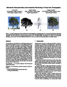
Figure 1: iWalk can preprocess a 13-million-triangle model in 17 minutes, and then render it with 98% accuracy at 9 frames per second on an inexpensive PC. Model courtesy of UNC Chapel Hill.

operations. A rendering thread uses a from-point visibility algorithm to find the nodes of the model hierarchy that the user sees, and sends fetch requests to a geometry cache, which reads nodes from disk into memory. To avoid bursts of disk operations, a lookahead thread uses a from-point visibility algorithm to find the nodes the user is likely to see next, and sends prefetch requests to the geometry cache. The system can run in approximate mode for interactive rendering, or in conservative mode for rendering with guaranteed accuracy. Using an inexpensive single-processor PC, iWalk can preprocess a model with tens of millions of polygons in a few minutes, and then render it at interactive frame rates (Figure 1). The main contributions of this paper are: • A system that can render a model with tens of millions of polygons at interactive frame rates on an inexpensive PC. • An incremental and fast out-of-core algorithm that builds an on-disk hierarchical representation for a large model. • A multi-threaded out-of-core rendering approach which to our knowledge is the first to combine speculative prefetching with a from-point occlusion-culling algorithm. The rest of this paper is organized as follows. Section 2 surveys related work. Section 3 presents the out-of-core preprocessing algorithm. Section 4 describes the out-of-core rendering approach. In Section 5, we present experimental results. In Section 6, we conclude and outline areas for future work.

2

Related Work

Researchers have studied the problem of rendering complex models at interactive frame rates for many years. Clark [12] proposed many of the techniques for rendering complex models used today, including the use of hierarchical spatial data structures, levelof-detail (LOD) management, hierarchical view-frustum and occlusion culling, and working-set management (geometry caching). Garlick et al. [21] presented the idea of exploiting multiprocessor graphics workstations to overlap visibility computations with rendering. Airey et al. [2] described a system that combined LOD management with the idea of precomputing visibility information for models made of axis-aligned polygons. Funkhouser et al. [20] described the first published system that supported models larger than main memory, and performed speculative prefetching. Their system was based on the from-region visibility algorithm of Teller and Séquin [32], which required long preprocessing times, and was limited to models made of axis-aligned cells. The iWalk system we present here is based on the from-point visibility algorithm of Klosowski and Silva [22, 23], which requires very little preprocessing, and can handle any 3D polygonal model. Aliaga et al. [3] presented the Massive Model Rendering (MMR) system, which employed many acceleration techniques, including replacing geometry far from the user’s point of view with imagery, occlusion culling, LOD management, and from-region prefetching. MMR was the first published system to handle models with tens of millions of polygons at interactive frame rates. A difference between MMR and iWalk is that MMR’s preprocessing step required user intervention, and took weeks to run, while iWalk’s preprocessing step is fully automatic, and takes minutes to run. Another difference is that MMR required an expensive high-end multi-processor graphics workstation, while iWalk runs on an inexpensive PC. Wald et al. [35] developed a ray tracing system that used a cluster of 7 dual-processor PCs to render low-resolution images of models with tens of millions of polygons at interactive frame rates. Their system could preprocess the UNC power plant model [36] in 2.5 hours (two orders of magnitude faster than MMR [3]). Our preprocessing algorithm is similar to the one of Wald et al., but our algorithm performs many fewer disk operations, and can preprocess the UNC power plant in 17 minutes. Avila and Schroeder [6] and El-Sana and Chiang [16] developed systems for interactive out-of-core rendering based on LOD management, but these systems did not perform occlusion culling. Varadhan and Manocha [34] describe a system for out-of-core rendering that uses hierarchical LODs [18] and prefetching, but their system does not perform occlusion culling, and their preprocessing step is in-core. Many other researchers [9, 10, 13, 27, 30, 31] have developed systems for out-of-core rendering and visualization. Ueng et al. [33] presented an out-of-core algorithm to build an on-disk octree for large unstructured tetrahedral meshes. Both their algorithm and ours save the structure (or skeleton) of the octree in a file, and the contents of the octree nodes in seperate files. Also, both algorithms enforce a maximum amount of data per octree node. The difference is that their algorithm may need to perform multiple passes over the same octree node during insertion, while our algorithm only needs one pass per node. Cignoni et al. [11] developed an out-of-core algorithm for simplification of large models. Their algorithm first builds a raw (not indexed) octree-based external memory mesh (OEMM), and then traverses the raw OEMM twice to build an indexed OEMM. Our preprocessing algorithm is similar to the first phase of their simplification algorithm. The main difference is that they build the octree starting from the leaves at a predefined depth, and then merge adjacent leaves with few triangles. We build the octree starting from the root, and then split leaves with too many triangles. Our algorithm and theirs have similar running times.

Wonka et al. [37] presented a from-region visibility preprocessing algorithm with occluder fusion. Their algorithm took 9 hours to preprocess a model with 8 million triangles, and was limited to 2.5D environments. In later work, Wonka et al. [38] employed a from-point approach that needed very little preprocessing, and used 2 processors to overlap visibility computation and rendering at runtime (similarly to the idea introduced by Garlick et al. [21]). But Wonka et al. [38] only reported results for 2.5D environments that were smaller than main memory. Durand et al. [15] presented a from-region visibility preprocessing algorithm that could handle 3D environments, as opposed to 2.5D [37]. But the algorithm took 33 hours to process a model with 6 million triangles. Schaufler et al. [29] also presented a fromregion 3D visibility preprocessing algorithm, but their largest test model had only 0.6 million triangles.

3

Out-Of-Core Preprocessing

Recall that our goal is to render a large model using an inexpensive PC with small memory. Our approach is to construct an outof-core hierarchical representation for the model at preprocessing time, and at runtime load on demand the hierarchy nodes that the user sees. The database literature uses the term bulk loading to refer to the construction of out-of-core spatial data structures. Agarwal et al. [1] and Arge et al. [5] present bulk loading algorithms for many data structures, including kd-trees, quad-trees, and R-trees. The algorithm we present here builds an out-of-core octree [28] whose leaves contain the geometry of the model. To store the octree on disk, our algorithm saves the geometric contents of each octree node in a separate file, and creates a hierarchy structure (HS) file (Figure 2). The HS file has information about the spatial relationship of the nodes in the hierarchy, and for each node it contains the node’s bounding box and auxiliary data needed for visibility culling. The HS file is the main data structure that the iWalk system uses to control the flow of data. A key assumption we make is that the HS file fits in memory. That is usually a trivial assumption. For example, the size of the HS file for a 13-million-triangle model is only 1 MB.

node structure id min point max point octant depth is leaf # vertices # triangles

hierarchy structure file

node contents files

node contents # vertices # vertex normals # vertex colors # triangles

...

...

vertices vertex normals vertex colors triangles

Figure 2: The on-disk hierarchical representation of a model. The out-of-core preprocessing algorithm builds an octree for a model, saving the skeleton of the octree in the hierarchy structure (HS) file, and the geometric contents of each node in a separate file. An in-core approach to build an octree for a model would process the entire model in one pass, using a machine with large enough memory to hold both the model and the resulting octree. We avoid this brute-force approach, because we do not want to use a separate expensive machine with large memory just to build the octree.

Our out-of-core algorithm builds an octree for a model directly on machines with small memory. The algorithm first breaks the model in sections that fit in main memory, and then incrementally builds the octree on disk, one pass for each section, keeping in memory only the section being processed. The out-of-core algorithm to build an octree for a model M with bounding box b and a maximum number V of vertices per leaf is: O CTREE -B UILD(M, b, V ) 1 break model M in sections S that fit into main memory 2 pick a section si ∈ S 3 O CTREE -I NIT(si , b, V ) 4 for each section s j ∈ S, s j 6= si 5 O CTREE -A DD -S ECTION(s j , V ) Breaking the model in sections is simple. Let N be the number of triangles in the model, and n the number of triangles that a machine can hold in memory (typically, N is much larger than n). We can create dN/ne sections of at most n triangles each, without bringing the entire model into memory, by reading at most n triangles at a time, and writing them to a separate file. Chiang et al. [10] propose a technique that splits the model in spatially coherent sections. To initialize the octree, we pick a section of the model, and insert the vertices and triangles of the section into the octree. The octree starts out as a single leaf that contains the bounding box of the model. We first insert the vertices of the section in the octree. For each vertex of the section, we find the leaf that contains the vertex, and add the vertex to the leaf’s list of vertices. If the number of vertices in the leaf exceeds the predefined limit, we create eight children under the leaf, and redistribute its vertices among its children. We then insert the triangles of the section in the octree. For each triangle of the section, we find the leaves touched by the triangle, and replicate the triangle in all those leaves, checking the limit of vertices per node. The final leaves may have different sizes, but each leaf will contain at most the predefined number of vertices. The routines to initialize an octree with a model section s are: O CTREE -I NIT(s, b, V ) 1 root ← new octree node with bounding box b 2 for each vertex v of model section s 3 O CTREE -N ODE -I NSERT-V ERTEX(root, v, V ) 4 for each triangle t of model section s 5 O CTREE -N ODE -I NSERT-T RIANGLE(root, t, V ) 6 save octree to disk O CTREE -N ODE -I NSERT-V ERTEX(x, v, V ) 1 if node x is not a leaf 2 y ← child of x containing vertex v 3 O CTREE -N ODE -I NSERT-V ERTEX(y, v, V ) 4 else 5 add vertex v to the list of vertices of node x 6 if the number of vertices in x is greater than V 7 create eight children under x 8 distribute the vertices in x among the children of x O CTREE -N ODE -I NSERT-T RIANGLE(x, t, V ) 1 if node x is a leaf 2 add triangle t to the list of triangles in x 3 if the number of vertices in x is greater than V 4 create eight children under x 5 distribute the triangles in x among the children of x 6 else 7 for each child y of node x touched by triangle t 8 O CTREE -N ODE -I NSERT-T RIANGLE(y, t, V ) After initializing the octree with one of the model sections, we add the other sections one at a time. To add a section to an octree,

we first read the the HS file (Figure 2) from disk. Recall that the HS file trivially fits in memory. We do not read the contents of any node yet. At this point, all the octree nodes in memory are empty, even the leaves that do have contents stored on disk. We then read the section itself, which by construction fits in memory, and insert the geometry of the section into the octree. After these insertions, some leaves will have received new data. Because of the limit of vertices per leaf, some leaves may have become internal nodes, and new leaves may have been created. For each old leaf modified by the insertions, we read the old contents from disk, reinsert the old contents into the old leaf, and update the contents of the old leaf on disk. The important point is that these reinsertions are local to the old leaf, and therefore never require reading more than one octree node of a fixed maximum size from disk. If the old leaf is now an internal node, its contents have been redistributed to its descendants; we then delete the file for the old leaf, and create new files for the new descendants. After updating each contents file, we free the memory allocated for it. Finally, we update the HS file on disk, and free the memory used by the model section and by the HS file. Thus, the routine to add a section s to an octree is: O CTREE -A DD -S ECTION(s, V ) 1 read octree structure (HS file) from disk 2 read model section s from disk 3 for each vertex v of model section s 4 O CTREE -N ODE -I NSERT-V ERTEX(root, v, V ) 5 for each triangle t of model section s 6 O CTREE -N ODE -I NSERT-T RIANGLE(root, t, V ) 7 for each old leaf x that was modified 8 read old contents of x from disk 9 reinsert old contents into x 10 if x is no longer a leaf 11 remove old contents file for x 12 for each leaf y descendant of x 13 update the contents file for y 14 free memory used by y 15 update HS file on disk 16 free memory used by section s 17 free memory used by HS file If the new section does not fit inside the bounding box of the original model, and we do not want to rebuild the octree for the entire model, we grow the octree toward the new section. We create seven siblings for the current root node, and a new root that will be the parent of the old root and its new siblings. We repeat this until the octree does contain the new section, and then proceed with the insertion as before. Our preprocessing algorithm has three important features: • It is an out-of-core algorithm. When processing a section, we only need enough memory to hold the section itself, the octree structure (the HS file), and the contents of one octree leaf. The section fits in memory by construction, the size of HS file is negligible, and the size of the contents of a leaf is limited by the maximum number of vertices per leaf. Therefore, we can create octrees for extremely large data. • It is an incremental algorithm. If new objects are added to the model, only the spatial regions touched by those objects need to be updated, as opposed to rebuilding the entire hierarchy. This is particularly useful for applications that build models incrementally, such as 3D scanning. • It is fast. For each section, it only reads a modified node once, doing the insertion in the most efficient way. Our algorithm builds the octree for the UNC power plant in just 17 minutes.

approximate visible set user interface (a)

camera

approximate visibility: PLP front (b)

nodes to render conservative conservative visible set visibility: cPLP (c)

rendering (d)

fetch request

predicted camera approximate approximate visibility: PLP visible set (h)

graphics card (e)

image

monitor (f)

fetch request

prefetch request

look−ahead (g)

nodes to render

geometry cache (i)

geometry read request geometry

disk (j)

Figure 3: The multi-threaded out-of-core rendering approach of the iWalk system. For each new camera (a), the system finds the set of visible nodes using either approximate visibility (b), or conservative visibility (c). For each visible node, the rendering thread (d) sends a fetch request to the geometry cache (i), and then sends the node to the graphics card (e). The look-ahead thread (g) predicts future cameras, estimates the nodes that the user would see then (h), and sends prefetch requests to the geometry cache (i).

4

Out-Of-Core Rendering

Thus far, we have shown iWalk’s preprocessing algorithm to create an out-of-core octree for a model larger than main memory. We now present iWalk’s out-of-core rendering approach that loads on demand the octree nodes that the user sees.

Overview of the Rendering Approach Figure 3 shows a diagram of iWalk’s rendering approach. The user interface (a) keeps track of the position, orientation, and field-ofview of the user’s camera. For each new set of camera parameters, the system computes the visible set — the set of octree nodes that the user sees. According to the user’s choice, the system can compute an approximate visible set (b), or a conservative visible set (c). To compute an approximate visible set, iWalk uses the prioritizedlayered projection (PLP) algorithm [22]. To compute a conservative visible set, iWalk uses cPLP [23], a conservative extension of PLP. (We will review PLP and cPLP shortly.) For each node in the visible set, the rendering thread (d) sends a fetch request to the geometry cache (i), which will read the node from disk (j) into memory. The rendering thread then sends the node to the graphics card (e) for display (f). To avoid bursts of disk operations, the look-ahead thread (g) predicts where the user’s camera is likely to be in the next few frames. For each predicted camera, the look-ahead thread uses PLP (h) to estimate the visible set, and then sends prefetch requests to the geometry cache (i).

Review of the PLP and cPLP Algorithms To better understand iWalk’s rendering approach, we need to review the visibility algorithms that iWalk uses. In approximate mode, iWalk uses the prioritized-layered projection (PLP) algorithm [22]. In conservative mode, iWalk uses the cPLP algorithm [23]. PLP is an approximate, from-point visibility algorithm that may be understood as a set of modifications to the traditional hierarchical view frustum culling algorithm [12]. First, instead of traversing the model hierarchy in a predefined order, PLP keeps the hierarchy leaf nodes in a priority queue called the front (Figure 3b), and traverses the nodes from highest to lowest priority. When PLP visits a node, it adds the node to the visible set, removes the node from the front, and adds the unvisited neighbors of the node to the front. Second, instead of traversing the entire hierarchy, PLP works on a

Figure 4: A section of the Soda Hall model. At runtime, the iWalk system uses the prioritized-layered projection (PLP) algorithm to estimate the nodes potentially visible from the current view frustum (outlined in yellow). The transparent color of each node indicates the projection priority of the node. Model courtesy of UC Berkeley.

budget, stopping the traversal after a certain number of primitives have been added to the visible set. Finally, PLP requires each node to know not only its children, but also all of its neighbors. An implementation of PLP may be simple or sophisticated, depending on the heuristic to assign priorities to each node. Several heuristics precompute for each node a value between 0.0 and 1.0 called solidity, which estimates how likely it is for the node to occlude an object behind it. At run time, the priority of a node is found by initializing it to 1.0, and attenuating it based on the solidity of the nodes found along the traversal path to the node (Figure 4). A key feature of PLP that iWalk exploits is that PLP can generate an approximate visible set based on just the information stored in the hierarchy structure (HS) file created at preprocessing time (Figure 2). In other words, PLP can estimate the visible set without access to the actual scene geometry.

Although PLP is in practice quite accurate for most frames, it does not guarantee image quality, and some frames may show objectionable artifacts. To avoid this potential problem, the system may optionally use cPLP [23], a conservative extension of PLP that guarantees 100% accurate images. But cPLP cannot find the visible set from the HS file only, and needs to read the geometry of all potentially visible nodes. The additional disk operations make cPLP much slower than PLP. Recall that PLP keeps the octree nodes in a priority queue called the front, and traverses the nodes from highest to lowest priority, adding nodes to the visible set up to a predefined budget of primitives. The cPLP algorithm augments the approximate visible set found by PLP into a conservative one (Figure 3c). There are many ways to implement cPLP [23], including using hardware-dependent extensions for visibility computation. Our implementation of cPLP uses an item-buffer technique that is portable to any system that supports OpenGL. Thus, cPLP needs to fetch geometry from the geometry cache (Figure 3i), and read pixels from the graphics card (Figure 3e).

The Geometry Cache To render a model larger than main memory, the iWalk system keeps on disk an octree-based representation for the model (Figure 2), and loads on demand the contents of the octree nodes that the user sees. Because nodes that are visible in one frame tend to be visible in the next frame (frame-to-frame coherence), iWalk tries to reduce the number of disk operations by maintaining a geometry cache (Figure 3i) with the contents of the most recently used nodes. As the user walks through a model, the conservative visibility thread (Figure 3c) and the rendering thread (Figure 3d) send fetch requests to the geometry cache (Figure 3i). A fetch request contains the identification of an octree node whose contents will be rendered. The geometry cache puts the fetch requests in a queue, and a set of fetch threads process the requests. (Butenhof [8] uses the term work queue to refer to a set of threads that accept work requests from a common queue, processing them potentially in parallel.) Each fetch thread pops a request from the fetch queue, and checks whether the contents of the requested node is in memory (a hit) or not (a miss). In the case of a miss, the fetch thread allocates memory for the contents of the requested node, and reads it from disk (Figure 3j). If the cache is full, the least recently used nodes are evicted from memory. Finally, the fetch thread puts the requested node in a queue for nodes that are ready to be rendered. Since the cost of disk read operations is high, most systems try to overlap these operations with other computations by running several processes on a multiprocessor machine [3, 19, 21], or on a network of machines [35, 38]. Along these same lines, our system uses threads on a single processor machine to overlap disk operations with visibility computations and rendering. The user can configure the number of threads that process the requests in the fetch queue. One advantage of using multiple fetch threads is that it avoids stalls in the rendering pipeline: if a fetch thread processes a miss, that thread will wait until the requested node is read from disk, but the fetch threads that process hits will put the requested nodes in the ready queue, keeping the graphics card busy. Another advantage of using multiple fetch threads is that it gives the operating system kernel a chance to better schedule the read operations when there are concurrent misses. The geometry cache uses a locking mechanism to prevent multiple threads from modifying or deleting the same node at the same time. The locking mechanism is similar to the one used by the UNIX operating system in its buffer cache [7]. The main difference is that the UNIX buffer cache uses multiple processes for parallelism and signals for synchronization, and we use threads and condition variables [8]. Another difference is that the UNIX buffer cache uses buffers of fixed size, and we use buffers of variable size.

The From-Point Prefetching Method The idea behind prefetching is to predict a set of nodes that the user is likely to see next, and bring them to memory ahead of time. Ideally, by the time the user sees those nodes, they will be already in the geometry cache, and the frame rates will not be affected by the disk latency. Many previous systems [3, 19, 20, 34] have used prefetching successfully. To our knowledge, all previous prefetching methods that employ occlusion culling have been based on from-region visibility algorithms, and were designed to run on multiprocessor machines. Our prefetching method works with from-point visibility algorithms, and runs as a separate thread in a uniprocessor machine. Our prefetching method exploits the fact that PLP can very quickly compute an approximate visible set. Given the current camera (Figure 3a), the look-ahead thread (Figure 3g) predicts future cameras based on the current camera’s position, linear speed, and angular speed. More sophisticated prediction schemes could consider accelerations and more than one past camera. For each predicted camera, the look-ahead thread uses PLP (Figure 3h) to determine which nodes the predicted camera is likely to see. For each node likely to be visible, the look-ahead thread sends a prefetch request to the geometry cache (Figure 3i). The geometry cache puts the prefetch requests in a queue (different from the fetch queue we described above), and a set of prefetch threads process the requests. If there are no fetch requests pending, and if the maximum amount of geometry that can be prefetched per frame has not been reached, a prefetch thread will pop a request from the prefetch queue, and read the requested node from disk (Figure 3j), without changing the node’s priority for replacement. Figure 5a shows the user’s view of the UNC power plant model [36] during a walkthrough session, and Figure 5b shows the state of the octree nodes in the geometry cache. Unlike our from-point prefetching method, from-region prefetching methods decompose the model into cells, and precompute for each cell the geometry that the user would see from any point in the cell. At runtime, from-region methods guess in which cell the user will be next, and load the geometry visible from that cell ahead of time. Our from-point prefetching method has several advantages over from-region prefetching methods. First, from-region methods typically require long preprocessing times (tens of hours), while our from-point method requires little preprocessing (a few minutes). Second, the set of nodes visible from a single point is typically much smaller than the set of nodes visible from any point in a region. Thus, our from-point prefetching method avoids unnecessary disk operations, and has a better chance than a from-region method of prefetching nodes that actually will be visible soon. Third, some from-region methods require that cells coincide with axis-aligned polygons in the model. Our from-point method imposes no restriction on the model’s geometry. Finally, the nodes visible from a cell may be very different from the nodes visible from a neighbor of that cell. Thus, a from-region method may cause bursts of disk activity when the user crosses cell boundaries, while a from-point method better exploits frame-to-frame coherence.

5

Experimental Results

To evaluate our system, we measured the preprocessing time and the runtime frame-rates for the 13-million-triangle UNC power plant model [36]. To our knowledge, no other system has been able to render this model at interactive rates on a single PC.

Preprocessing Results We measured the time to preprocess the power plant model on a computer with a 900 MHz AMD Athlon CPU, 512 MB of main memory, and a 400 GB SCSI disk. The computer’s operating system was Red Hat Linux 7.2.

(a) user’s view

(b) cache view

Figure 5: A sample frame inside the power plant model. (a) The image that the user sees. (b) The state of the nodes in the geometry cache.

The power plant model consists of 21 sections, each of which fits in the main memory of the test machine. We used our out-of-core incremental algorithm to build the octree for the entire model, one section at a time. We set a limit of 15,000 vertices per leaf, and the resulting octree had 14, 722 leaves. The size of the hierarchy structure (HS) file (Figure 2) was 1 MB, and the size of the largest contents file was 600 KB. Thus, after the octree was created, even a machine with small memory could use them for rendering. Recall that being able to keep the HS file in memory is critical for the incremental construction of the octree, and for the use of the PLP algorithm for approximate visibility computation. The total preprocessing time was 17 minutes, and the maximum amount of memory the preprocessing algorithm ever needed was 214 MB, even though the final size of the octree was 2.2 GB. If the test machine had less memory than 214 MB, we would have broken the model down into smaller pieces (Section 3). The important point is that we were able to quickly build a large octree using a modest PC with small memory. The original model has 13 million triangles, while the final octree has 18 million triangles, because the preprocessing algorithm replicates a triangle in all leaves the triangle touches. The average replication factor was thus 1.5. The disk size of the original model was 0.6 GB, while the disk size of the final octree was 2.2 GB. The octree needs more disk space not only because of the replicated triangles, but also because of the vertex normals, which are stored in the octree, but not in the original model. Storing the normals on disk instead of computing them at runtime is a time-space tradeoff.

Runtime Results For the runtime tests, we used a computer with a 900 MHz AMD Athlon CPU, 128 MB of main memory, a 30 GB IDE disk, and an nVidia GeForce2 graphics card. The computer’s operating system was Red Hat Linux 7.2. Using top, we found that the operating

system and related utilities (including the X server) uses roughly 64 MB of main memory when idle. The user can configure many parameters in our system, including geometry cache size, number of fetch threads, number of prefetch threads, maximum amount of prefetched geometry per frame, visibility mode (approximate or conservative), target frame rate, and image resolution. These parameters depend mainly on the triangle throughput of the graphics card and the disk bandwidth. For our test machine, we found that this configuration works well in practice: 32 MB of geometry cache, 8 fetch threads, 1 prefetch thread, a maximum of 1 MB of prefetched geometry per frame, approximate visibility with a budget of 140,000 triangles per frame, a target frame rate of 10 fps, and image resolution of 1024×768. To analyze the overall performance of our system, we measured the frame rates the system achieved when walking through the power plant model along a large path of 36,432 viewpoints. The path visits almost every part of the model, and requires fetching a total of 1.6 GB of data from disk. Using the configuration described above, our system rendered the frames along that path in less than 1.5 hours. The use of approximate visibility causes objects to pop in and out of view occasionally because of visibility computation mistakes, but objectionable artifacts were rare. Only 147 frames (0.4%) caused the system to achieve less than 1 fps. The mean frame rate was 8.3 fps, and the median frame rate was 9.1 fps. These frame rates are close to the target of 10 fps. To analyze the detailed performance of our system, it is easier to use shorter paths. For this purpose, we used a 500-frame path which required 210 MB of data to be read from disk. If fetched independently, the maximum amount of memory necessary to render any given frame in approximate mode would be 16 MB. To study how multiple threads improve the frame rates, we ran tests using three different configurations. The first configuration is entirely sequential: a single thread is responsible for computing visibility, performing disk operations, and rendering. The second

1.0 0.8 accuracy 0.4 0.6 0.2

12 frame rate (frames/sec) 2 4 6 8 10

0.0

100

0

0 0

100

200 300 frame number

400

500

400

500

Figure 7: Image accuracy for a 500-frame walkthrough of the power plant model when using approximate visibility. The vertical axis represents the fraction of correct pixels in the approximate images in comparison to the conservative images. The minimum accuracy was 89%, and the median accuracy was 98%.

0

frame rate (frames/sec) 2 4 6 8 10

12

(a) sequential fetching and rendering


0

100


400

500

0


12

(b) concurrent fetching and rendering

0

100


400

500

(c) concurrent fetching, rendering, and prefetching

Figure 6: Using multiple threads to improve frame rates. We measured the frame rates during a 500-frame walkthrough of the power plant model under three configurations: (a) using one thread for fetching and rendering; (b) using multiple threads to overlap fetching and rendering; and (c) using multiple threads to overlap fetching, rendering, and prefetching. Concurrent fetching eliminates some downward spikes, and adding concurrent speculative prefetching eliminates almost all of the remaining spikes. The first spike happens because the cache is initially empty. The three configurations produce identical images.

configuration adds asynchronous fetching to the first configuration, allowing up to 8 fetch threads. The third configuration adds an extra thread for speculative prefetching to the second configuration, allowing up to 1 MB of geometry to be prefetched per frame. Figure 6 shows the frame rates achieved by these three configurations for the 500-frame path. For the purely sequential configuration, we see many downward spikes that correspond to abrupt drops in frame rates, which are caused by the latency of the disk operations, and spoil the user’s experience. When we add asynchronous fetching, most of the downward spikes disappear, but many still remain. The user’s experience is much better, but the frame rate drops are still disturbing. When we add speculative prefetching, almost all downward spikes disappear, and the user experience is smooth. Note that the gain in interactivity comes entirely from overlapping the independent operations. The three configurations achieve exactly the same image accuracy (Figure 7). We could obtain further gains in interactivity if we were willing to compromise image quality [19]. Figure 8 shows why prefetching improves the frame rates. The charts compare the amount of geometry that the system reads from disk per frame for the second and third configurations described above. Prefetching greatly reduces the need to fetch large amounts of geometry in a single frame, and thus helps the system to maintain higher and smoother frame rates. Figure 9 shows that the user speed is another important parameter in the system, and has to be adjusted to the disk bandwidth. When the user speed increases, the changes in the visible set are larger. In other words, as the frame-to-frame coherence decreases, the amount of data the system needs to read per frame increases. Thus, caching and prefetching are more effective if the user moves at speeds compatible with the disk bandwidth. The figure also indicates that higher disk bandwidth should improve frame rates.

6

Conclusion

We have presented iWalk, a system for rendering large models on machines with small memory at interactive frame rates. Given a model, the system uses a new out-of-core preprocessing algorithm to quickly build an octree-based representation for the model on disk. At runtime, the system uses a new out-of-core rendering approach that loads on demand the octree nodes that the user sees. The rendering approach uses multiple threads in a single processor to overlap visibility computations, disk operations, and rendering. The system can run in approximate mode (using the PLP algorithm) for interactive rendering, or in conservative mode (using the cPLP

8000

8000

2000

size (KB) 4000 6000

misses prefetches

0

0

2000

size (KB) 4000 6000

misses prefetches

0

100


400

500

0

100

(a) without prefetching


400

500

(b) with prefetching

12 frame rate (frames/sec) 2 4 6 8 10 0

0


12

Figure 8: Using prefetching to amortize the cost of disk operations. We measured the amount of geometry fetched per frame without prefetching (a) and with prefetching (b). Prefetching amortizes the cost of bursts of disk operations over frames with few disk operations, thus eliminating or alleviating most frame rate drops. The system was configured to prefetch at most 1 MB per frame.

0

20

40

60 80 frame number

100

120

0


200

250

800

1000

frame rate (frames/sec) 2 4 6 8 10 0

0


12

(b) high user speed

12

(a) very high user speed

50

0

100


(c) normal user speed

400

500

0

200


(d) low user speed

Figure 9: Adjusting the user speed to the disk bandwidth. We measured the frame rates along a camera path inside the power plant model for different user speeds (or equivalently, for different number of frames in the path). If the user moves too fast, the frame rates are not smooth. The faster the user moves, the larger the changes in occlusion, and therefore the larger the number of disk operations.

algorithm) for rendering with guaranteed accuracy. A key component of the rendering approach is the geometry cache, which maintains a fetch queue for nodes that will be rendered in the current frame, and a prefetch queue for nodes that are likely to be rendered in future frames. The prefetch queue receives requests from a look-ahead thread that uses the PLP algorithm to estimate future visible sets. We believe our system is the first to employ a prefetching method based on a from-point visibility algorithm. The system can preprocess the 13-million-triangle UNC power plant model in 17 minutes, and then render it with 98% accuracy at 9 frames per second using an inexpensive PC. To our knowledge, our system is the first to render a model this large on an inexpensive PC. There are several possible areas for future work. One is adding level-of-detail (LOD) management [4, 12, 14, 17, 20, 24, 25, 26] to our system. In approximate mode, our system may produce images with low accuracy if the camera sees the entire model. El-Sana et al. [17] show how to integrate LOD management with PLP-based occlusion culling. Although this integration is highly desirable, because it can improve rendering quality, it will come at the expense of a more expensive preprocessing step and a more complex rendering algorithm. Another possible area for future work is speeding up rending in conservative mode, which currently can be much slower than rendering in approximate mode. Part of the problem is the lack of good occlusion query functionality in current hardware, while another part is that conservative rendering significantly raises the disk bandwidth requirements. Finally, we also would like to extend the system to support dynamic scenes.

Acknowledgements We thank Daniel Aliaga, David Dobkin, Juliana Freire, Thomas Funkhouser, Jeff Korn, Patrick Min, and Emil Praun for suggestions and encouragement. We also thank the University of North Carolina at Chapel Hill and the University of California at Berkeley for providing us with datasets. Good models “are at least as valuable as the visible surface algorithms that render them [12].” This research was partly funded by CNPq (Conselho Nacional de Desenvolvimento Cient´ıfico e Tecnológico), Brazil.

References [1] P. Agarwal, L. Arge, O. Procopiuc, and J. Vitter. A framework for index bulk loading and dynamization. In International Colloquium on Automata, Languages, and Programming, pages 115–127, 2001. [2] J. M. Airey, J. H. Rohlf, and J. Frederick P. Brooks. Towards image realism with interactive update rates in complex virtual building environments. 1990 ACM Symposium on Interactive 3D Graphics, 24(2):41–50, Mar. 1990. [3] D. Aliaga, J. Cohen, A. Wilson, H. Zhang, C. Erikson, K. Hoff, T. Hudson, W. Stürzlinger, E. Baker, R. Bastos, M. Whitton, F. Brooks, and D. Manocha. MMR: An interactive massive model rendering system using geometric and image-based acceleration. 1999 ACM Symposium on Interactive 3D Graphics, pages 199–206, Apr. 1999. [4] C. Andújar, C. Saona-Vázquez, I. Navazo, and P. Brunet. Integrating occlusion culling and levels of detail through hardlyvisible sets. Computer Graphics Forum, 19(3):499–506, 2000. [5] L. Arge, K. Hinrichs, J. Vahrenhold, and J. Vitter. Efficient bulk operations on dynamic R-trees. In Proc. Workshop on Algorithm Engineering, pages 104–128, 1999.

[6] L. S. Avila and W. Schroeder. Interactive visualization of aircraft and power generation engines. In IEEE Visualization ’97, pages 483–486. IEEE, Nov. 1997. [7] M. J. Bach. The Design of the UNIX Operating System. Prentice Hall, 1986. [8] D. R. Butenhof. Programming with POSIX Threads. Addison Wesley, 1997. [9] Y.-J. Chiang and C. T. Silva. I/O optimal isosurface extraction. IEEE Visualization ’97, pages 293–300, Nov. 1997. [10] Y.-J. Chiang, C. T. Silva, and W. J. Schroeder. Interactive outof-core isosurface extraction. IEEE Visualization ’98, pages 167–174, Oct. 1998. [11] P. Cignoni, C. Rocchini, C. Montani, and R. Scopigno. External memory management and simplification of huge meshes. IEEE Transactions on Visualization and Computer Graphics, 2002. To appear. [12] J. H. Clark. Hierarchical geometric models for visible surface algorithms. Communications of the ACM, 19(10):547–554, Oct. 1976. [13] M. B. Cox and D. Ellsworth. Application-controlled demand paging for out-of-core visualization. IEEE Visualization ’97, pages 235–244, Nov. 1997. [14] M. A. Duchaineau, M. Wolinsky, D. E. Sigeti, M. C. Miller, C. Aldrich, and M. B. Mineev-Weinstein. ROAMing terrain: Real-time optimally adapting meshes. In IEEE Visualization ’97, pages 81–88. IEEE, Nov. 1997. [15] F. Durand, G. Drettakis, J. Thollot, and C. Puech. Conservative visibility preprocessing using extended projections. In Proceedings of Siggraph 2000, pages 239–248, July 2000. [16] J. El-Sana and Y.-J. Chiang. External memory viewdependent simplification. Computer Graphics Forum, 19(3):139–150, Aug. 2000. [17] J. El-Sana, N. Sokolovsky, and C. T. Silva. Integrating occlusion culling with view-dependent rendering. In IEEE Visualization 2001, pages 371–378, Oct. 2001. [18] C. Erikson, D. Manocha, and W. V. Baxter III. HLODs for faster display of large static and dynamic environments. In 2001 ACM Symposium on Interactive 3D Graphics, pages 111–120, Mar. 2001. [19] T. A. Funkhouser. Database management for interactive display of large architectural models. Graphics Interface ’96, pages 1–8, May 1996. [20] T. A. Funkhouser, C. H. Séquin, and S. J. Teller. Management of large amounts of data in interactive building walkthroughs. 1992 ACM Symposium on Interactive 3D Graphics, 25(2):11– 20, Mar. 1992. [21] B. J. Garlick, D. R. Baum, and J. M. Winget. Interactive viewing of large geometric databases using multiprocessor graphics workstations. In Siggraph Course: Parallel Algorithms and Architectures for 3D Image Generation, pages 239–245. ACM Siggraph, 1990. [22] J. T. Klosowski and C. T. Silva. The prioritized-layered projection algorithm for visible set estimation. IEEE Transactions on Visualization and Computer Graphics, 6(2):108–123, Apr.-June 2000.

[23] J. T. Klosowski and C. T. Silva. Efficient conservative visibility culling using the prioritized-layered projection algorithm. IEEE Transactions on Visualization and Computer Graphics, 7(4):365–379, Oct.-Dec. 2001. [24] P. Lindstrom. Out-of-core simplification of large polygonal models. In Proceedings of Siggraph 2000, pages 259–262, July 2000. [25] P. Lindstrom, D. Koller, W. Ribarsky, L. F. Hughes, N. Faust, and G. Turner. Real-time, continuous level of detail rendering of height fields. In Proceedings of Siggraph 96, pages 109– 118. ACM Siggraph, Aug. 1996. [26] P. Lindstrom and C. T. Silva. A memory insensitive technique for large model simplification. In IEEE Visualization 2001, pages 121–126, Oct. 2001. [27] M. Pharr, C. Kolb, R. Gershbein, and P. Hanrahan. Rendering complex scenes with memory-coherent ray tracing. Proceedings of Siggraph 97, pages 101–108, Aug. 1997. [28] H. Samet. The Design and Analysis of Spatial Data Structures. Addison-Wesley, 1990. [29] G. Schaufler, J. Dorsey, X. Decoret, and F. X. Sillion. Conservative volumetric visibility with occluder fusion. In Proceedings of Siggraph 2000, pages 229–238, July 2000. [30] H.-W. Shen, L.-J. Chiang, and K.-L. Ma. A fast volume rendering algorithm for time-varying fields using a time-space partitioning (TSP) tree. IEEE Visualization ’99, pages 371– 378, Oct. 1999. [31] P. M. Sutton and C. D. Hansen. Accelerated isosurface extraction in time-varying fields. IEEE Transactions on Visualization and Computer Graphics, 6(2):98–107, Apr.-June 2000. [32] S. J. Teller and C. H. Séquin. Visibility preprocessing for interactive walkthroughs. Proceedings of Siggraph 91, 25(4):61–69, July 1991. [33] S.-K. Ueng, C. Sikorski, and K.-L. Ma. Out-of-core streamline visualization on large unstructured meshes. IEEE Transactions on Visualization and Computer Graphics, 3(4):370– 380, Oct.-Dec. 1997. [34] G. Varadhan and D. Manocha. Out-of-core rendering of massive geometric environments. In IEEE Visualization 2002. To appear. [35] I. Wald, P. Slusallek, and C. Benthin. Interactive distributed ray tracing of highly complex models. Rendering Techniques 2001, pages 277–288, 2001. [36] Walkthru Project at UNC Chapel Hill. Power plant model. http://www.cs.unc.edu/˜geom/Powerplant/. [37] P. Wonka, M. Wimmer, and D. Schmalstieg. Visibility preprocessing with occluder fusion for urban walkthroughs. In Rendering Techniques 2000, pages 71–82, 2000. [38] P. Wonka, M. Wimmer, and F. Sillion. Instant visibility. Computer Graphics Forum, 20(3):411–421, 2001.