IEEE TRANSACTIONS ON RELIABILITY, VOL. 60, NO. 1, MARCH 2011
41
Machine Condition Classification Using Deterioration Feature Extraction and Anomaly Determination Dongxiang Jiang and Chao Liu
Abstract—Condition classification has been widely used for assessing equipment status for machine condition monitoring and diagnostics. An engine was fitted with one temperature and two pressure sensors to study the machine conditions in prognostics with an added abnormal state, in addition to the conventional normal and failure states. This work enables a better classification capability in order to predict deterioration in the engine. Information related to three deterioration processes was collected, and preprocessed using singular point elimination, deviation value acquisition, and data normalization. Wavelet transforms were used to extract deterioration features with different mother tests to wavelets. The mother wavelets were selected using optimize the wavelet selection. The deterioration was related to the amount of anomaly, with the abnormal states defined to distinguish the functional from the failure states. A Learning Vector Quantization (LVQ) neural network was used to classify the machine conditions, including normal, abnormal, and failure states. The results showed that the deterioration features defined using the Daubechies wavelet (db8) most strongly correlated with the original signal, so that the classification accuracy based on the deterioration features was greatly improved. The LVQ classification system had good accuracy for machine condition classification, and was adaptable to various engine conditions. Index Terms—Condition classification, learning vector quantization neural network, test, wavelet transform.
ACRONYM CBM
Condition Based Maintenance
PM
Preventive Maintenance
AI
Artificial Intelligence
ARIMA
Autoregressive Integrated Moving Average
ARCH
Autoregressive Conditional Heteroscedastic
LVQ
Learning Vector Quantization
DWT
Discrete Wavelet Transform
CWT
Continuous Wavelet Transform
Manuscript received March 30, 2010; revised May 31, 2010, June 23, 2010 and July 19, 2010; accepted July 26, 2010. Date of publication January 28, 2011; date of current version March 02, 2011. This work was supported by the National Natural Science Foundation of China (Grant 60979014) and the National Basic Research Program of China (973 Program) (Grant 2007CB210304). Associate Editor: W. Wang. The authors are with the State Key Laboratory of Control and Simulation of Power System and Generation Equipment, Department of Thermal Engineering, Tsinghua University, Beijing 100084, P. R. China (e-mail: jiangdx@tsinghua. edu.cn;
[email protected]). Digital Object Identifier 10.1109/TR.2011.2104433
I. INTRODUCTION HE development of maintenance strategies has experienced three stages: breakdown maintenance, time-based maintenance, and condition-based maintenance (CBM) [1], [2]. Unlike breakdown and time-based maintenance, CBM seeks to achieve a better availability, and a higher safety and reliability. Therefore, CBM has attracted more attention [3]. Diagnostics and prognostics are two main objectives of CBM. Diagnostics is concerned with fault detection, fault isolation, and fault identification [2]; while prognostics focuses more on the possibility of fault occurrence in the future, and the remaining useful life by monitoring the material condition or function loss [4]. Thus, prognostics have attracted more attention in recent research, based on the assumption that failures are caused by component aging, and deterioration. Thus, condition monitoring can be used for failure onset extraction in mechanical systems [5], [6]. Several approaches have been proposed for prognostics, with model-driven, and data-driven methods being two of most important ones [7]–[9]. Model-driven prognostics, established with a mathematical model based on the underlying physics of components’ deterioration, is largely applied to specific equipment. As a result, model-driven prognostics has a relatively narrower application range, but with higher accuracy. Data-driven prognostics uses analyses of monitoring data during machine operations as well as history data, often using Artificial Intelligence (AI) [10]. The adaptability of data-driven prognostics may reduce model construction costs, but may also result in the loss of accuracy compared with model-driven prognostics, as the deterioration mechanism is not considered. Other prognostic methods have been studied with evolutionary prognostics as a new method to predict equipment failures, and failure probability. Evolutionary prognostic approaches can achieve a better performance when the failure is related to equipment degradation with function loss or parameter variations. Byington and Roemer [5] used an evolutionary approach for gas turbine compressor wash prognostics. Evolutionary prognostics analyses the deterioration to help the maintenance decision maker by predicting the equipment conditions, where the conditions are signified by the feature space related to the measured parameters. Condition classification using continuously monitored field data for diagnostics and prognostics is crucial for evaluating equipment status, and has been widely studied for machine condition monitoring and diagnostics [11]–[14]. In condition monitoring, the conditions are typically classified into normal, and various faulty types. Yang [12] used condition classification to study the healthy and faulty states in a small reciprocating compressor. One normal condition and four faulty conditions of the roller bearing were classified in [13]. In fault diagnostics,
T
0018-9529/$26.00 © 2011 IEEE
42
IEEE TRANSACTIONS ON RELIABILITY, VOL. 60, NO. 1, MARCH 2011
14 faulty types of the turbo pump were classified in [14], while normal states and abnormal states were not considered. In machine operation processes, once the machine departs from the normal state, there exists an intermittent state between the normal state and a failure state [15]. Usually the intermittent state has little effect on the machine, and may not cause significant function loss. How to estimate this abnormal state between the normal and failure states is an actual problem in prognostics. Anomaly determination is proposed in this paper to distinguish the abnormal state from the normal and failure states. The purpose is that, once the abnormal states can be defined and distinguished, they can predict the deterioration trends. Feature extraction approaches are necessary for the clarity of the deterioration trends because the measured parameters contain much information, along with noises and disturbances. Wavelet transforms are widely used in signal processing and fault diagnostics in many fields including feature extraction [16], [17], but have not been widely used to indicate equipment deterioration. It has been validated that wavelet transforms are better for the analysis of the non-stationary signals [18], where the signals in deterioration processes are typically non-stationary ones. Wavelet transforms use various kinds of mother wavelets [19]. Daubechies wavelets are frequently used for mother wavelets [20], [21], but the effectiveness of different mother wavelets needs to be validated in specific applications. Truchetet and Laligant [22] proposed criteria to choose the mother wavelets including the regularity, the number of vanishing moments, and the compactness. Other properties are needed to properly choose mother wavelets in situations that vary greatly in different applications. Rafiee [23] studied the use of mother wavelets for gear and bearing fault diagnostics including Haar wavelets, Daubechies wavelets, Coiflet wavelets, Morlet wavelets, and Meyer wavelets. The similarity between the results with each selected mother wavelet and the standard mother wavelet was used to evaluate the effectiveness [23], [24]. The paper presents a test to validate the correlation between the deterioration features and the original signals, with the probability of the test results as the criterion for the optimization of mother wavelets. The paper presents the definition of the normal, abnormal, and failure state through anomaly determination, and the condition classification through LVQ neural networks. The purpose is to distinguish various abnormal conditions between the normal and failure states to predict the deterioration trends. The remaining part of the paper is organized as follows. Section II presents the condition classification obtained by deterioration feature extraction based on the wavelet transform. A significance test is carried out to validate the correlation between the features and the original signals. The data acquisition, preprocessing and anomaly definitions are also presented. Section III discusses results of the feature extraction and condition classification presented in Section II. Finally, conclusions are given in Section IV. II. METHODS AND DATA During machine deterioration, failures may occur after a relatively long time, and the deterioration is indicated by changes of the performance and various measured parameters. The param-
Fig. 1. Multilevel decompositions in wavelet transform.
eters typically change continuously, and so does the deterioration. These characteristics can then be used to identify the equipment deterioration before failures occur. The condition monitoring system will use the measured parameters to identify these changes. Proper analytical methods for extracting the features from those parameters for an accurate deterioration detection are essential, and developed in this paper. A. Deterioration Feature Extraction Using Wavelet Transform As a machine deteriorates, changes in the parameters reflect the machine status, usually in monotonic or low frequency signals. Therefore, the parameter changes can be used to indicate the deterioration over time as the machine operates. Wavelet decomposition and reconstruction are used in this paper to extract the deterioration features from these parameters in three steps. First, the parameter signal is decomposed into four levels using Discrete Wavelet Transform (DWT). DWT, derived from the Continuous Wavelet Transform (CWT), is based on the discretization of the dilation factor, and the translation parameter. The deterioration features are extracted using the multilevel wavelet analysis illustrated in Fig. 1 to determine the detailed information in , and the approximation information in . Second, wavelet reconstruction is used to reconstruct the signal coefficients. As down sampling was used in the decomand the approximation position processes, details of have samples of which need to be reconstructed. The reconstruction of a single branch of details and approximation is implemented to acquire the low frequency component. Third, the deterioration feature is then extracted from the mulis then retilevel decomposition results. The information in lated to the deterioration. This analysis uses the Daubechies wavelets and the Coiflet wavelets to acquire the optimization of the mother wavelet. The Daubechies wavelets are a family of orthogonal wavelets characterized by a maximum number of vanishing moments for some given support [20]. The Coiflet wavelets are built from Daubechies with more symmetrical wavelet and scaling functions. B. Significance Test Before the extracted deterioration features are used for condition classification, significance tests are used to validate the correlation between the extracted features and the original signal. The correlation coefficient is usually based on the linear hypothesis. Then, the correlation coefficient is defined as [25] (1)
JIANG AND LIU: MACHINE CONDITION CLASSIFICATION
43
where is the correlation coefficient between and , is the covariance, is the standard deviation of , and is the standard deviation of . With these definitions, the correlation coefficient reflects the significance of the hypoth. It is therefore a linear regression test. esis However, because the high frequency components of the original signal are suppressed by the wavelet decomposition and reconstruction, the feature variance is then smaller than that of the original signal. A correlation coefficient that is much smaller than 1 only means that the relationship between the two samples is not linear, and the correlation coefficient is not suitable for the correlation in this paper. The test statistic represents the significance between the two samples, and is applied in this , and for paper. The test for the feature samples is . The null hypothesis for the the original signal is test is
TABLE I CLASSIFICATION CONDITIONS FOR THREE DETERIORATION PROCESSES
(2)
and has a good adaptability for complex bounds [31]. An LVQ neural network contains an input layer, a competitive layer, and an output layer. The input layer has the same number of nodes as the dimension of the input feature vector, the competitive layer contains the Kohonen neurons, and the output layer is linearly related to the competitive layer. In the training process of the LVQ neural network, the Euclidean distance from the input layer to the Kohonen layer is calculated as [32]
Then the test statistic can be calculated based on the Student’s test [26]
(6)
(3)
where is the mean of the residuals, is the number of samples, and is the standard deviation of the sample. With a large number of samples, the null hypothesis can be rejected if (4) indicates rejection of the null hypothesis Therefore, indicates a failure to at the 5% significance level, and reject the null hypothesis at the 5% significance level. When h is closer to zero, the null hypothesis is harder to reject with better correlation between the extracted deterioration feature, and the original signal. Then, the hypothesis for the mean value of the residuals is
The probability of the hypothesis given by the test is the . Larger indicates probability of rejecting the hypothesis a better correlation between the deterioration feature and the signal. C. Classification System The machine condition is classified based on the deterioration features. The normal states for the three deterioration processes considered in this paper are the same, while the abnormal and failure states differ. Thus, seven different conditions are classified in Table I, including one normal state, three abnormal states, and three failure states. The LVQ neural network is used to build the classification system. The LVQ is a class of learning algorithms for nearest prototype classification [27], [28] introduced by Kohonen [29], which has been widely used for pattern recognition in many areas [30],
where is the input vector, and is the weight vector of the competitive layer. The nearest node is determined to be the winner, and its weight vector is adjusted according to whether the winning node is in the class of the target output vector. • If the winner is the correct class, then (7) where is the learning parameter. • If the winner is not the correct class, then (8) where is the learning parameter. Many studies have shown the optimization approaches to achieve higher classification accuracies, such as the advanced training algorithm LVQ 2.1 [33]. Other approaches have also been developed, such as support vector machine [11], [12], [34]. However, the classification accuracy depends on the specific application. This analysis seeks to evaluate the effects of the deterioration feature extraction. The condition classification control experiments used the LVQ neural network with the training approach in (6) –(8) to analyze the effectiveness of the feature extraction approaches. Two-class LVQ classifiers were used for the condition classification system with 8 neurons in the competitive layer. D. Data Acquisition and Preprocessing The machine degradation data used in this paper is based on a 12 cylinder engine running in the field. The dynamic pressures are often used to signify the conditions and faults in the engine. Vibration signals from the shafts are also often used to reflect the faults responses in fault diagnostics [35]. Combinations of the temperatures, pressures, vibration signals, and other indicators are often used for fault identification and diagnostics due to the very complex nature of faults in engines. In this analysis, the
44
IEEE TRANSACTIONS ON RELIABILITY, VOL. 60, NO. 1, MARCH 2011
Fig. 3. Deviation value of setup 2. Fig. 2. Measured data for different setups for the same loads.
evaluations were based on one temperature, and two pressure parameters, defined as P1, P2, and P3. The fault analyses are based on deterioration data for three faults, including an exhaust valve fault, an injector fault, and an electro-magnetic valve fault. Respectively, the faults are defined as F1, F2, and F3; and the deterioration processes are defined as DP1, DP2, and DP3. The sample interval was five minutes, and the mean values were collected every five minutes. The original signals collected online contain noises and other disturbances, which complicates the extraction of the features. The original signals are preprocessed using singular point elimination, deviation value acquisition, and data normalization. Singularity detection is used first to eliminate singularities in the monitoring data. Because the parameters were measured in the field, the variations of the measured parameters are assumed to be continuous. With high sampling rate data, a numerical filter can be used to eliminate singular points. However, the data used here had low sampling rate, so a specific elimination method is required. Three steps are used here to eliminate singular points: 1) Threshold definition. Experience has shown that the threshold should be twice the maximum variation of the signal. 2) Search for the singular point. The measured data are evaluated to identify if any data exceeds the threshold. 3) Determine the substitution value. For data that exceed the threshold, a substitution value is generated based on the linear variation of the signal. Secondly, the difference between the deterioration component and normal component is calculated to derive the feature parameters. The measured values of parameter P2 shown in Fig. 2 are for three similar sets of instrumentation installed in the same engine. The setups were run at the same loads with setup 2 showing obvious deterioration during operation, which results in the variations of the measured parameters. Therefore, monitoring of the difference between the signal with the deteriorated component and the signal with the normal component can be used to indicate the extent of the degradation. The differences for setup 2 are shown in Fig. 3. Thirdly, the data are normalized based on the contributions of the different parameters to failures. The parameters’ variations
are quite large with different setups. Therefore, normalization is needed to generate a uniform deterioration feature space. for data normalization is defined The normalized variable as count (9) where
is the measured value of the th parameter at count , is the maximum value of the th parameter, and is the coefficient determined by the parameter’s impact on the fault occurrence. The signals for the three deterioration processes after the preprocessing are shown in Fig. 4. The original space used for condition classification is formed from the preprocessed signals. The preprocessed signals are then used for the feature extraction based on wavelet transforms, with the deterioration feature space formed from the deterioration features. E. Anomaly Determination The boundaries for the three conditions classified in a deterioration process were originally coterminous, with the abnormal state adjacent to the normal and failure states. The abnormal state is determined first, and then determine the boundaries for the three conditions. The feature vectors are formed from the measured parameters (10) where is the feature vector at count , and is the feature value of the th parameter at count . The anomaly degree is defined based on the machine degradation (11) where (12) (13) is the mean value vector of the normal state, and mean value of the th parameter in the normal state.
is the
JIANG AND LIU: MACHINE CONDITION CLASSIFICATION
45
Fig. 4. Data for three machine deterioration processes after data preprocessing.
Then the abnormal rule is determined as Normal Abnormal Failure
(14) (15) (16)
where (17) (18) is the mean value vector of the failure state, is the mean is the lower value of the th parameter in the failure state, limit of the abnormal state, and is the upper limit of the abnormal state. The lower, and upper limits were respectively selected as , and . Then, the training and test samples were formed. 400 training samples were used including 100 samples for the normal state, 50 samples for each abnormal state, and 50 samples for each failure state. Three deterioration processes were used as test samples, including 800 samples for DP1, 2460 samples for DP2, and 2164 samples for DP3. The same training and test samples were used for control experiments in different condition classification approaches. The time intervals of the samples were fixed even though the samples were to be processed using feature extraction approaches. III. RESULTS AND DISCUSSION A. Extracted Deterioration Features and Significance Test The feature extraction method was used with the multilevel wavelet decomposition with various mother wavelets. The
Fig. 5. Multilevel decompositions for parameter P1 in deterioration process DP1 using wavelet transforms.
signal from parameter P1 in deterioration process DP1 analyzed using db8 is used here as an example of the transform process. The multilevel decomposition results of parameter P1 in deterioration process DP1 are shown in Fig. 5, with four detail components in high frequency and one approximation component in low frequency.
46
IEEE TRANSACTIONS ON RELIABILITY, VOL. 60, NO. 1, MARCH 2011
Fig. 6. Extracted deterioration features for three deterioration processes using wavelet transform.
t
TABLE II TEST RESULT BETWEEN THE DETERIORATION FEATURES AND THE ORIGINAL SIGNAL
Fig. 7. Average probability of t test statistics for different mother wavelets.
The approximation component is selected as the most distinctive feature. The other datasets were processed with the same steps, with the feature extraction results shown in Fig. 6. The effectiveness and significance of the features identified using other mother wavelets were evaluated using the test statistics. The residuals between the original signal and the feature were again acquired using the signal for parameter P1 in deterioration process DP1 using db8 wavelet. The results in Table II show that the test result is 0.0705, and the result is 0.9438. The test results for other mother wavelets listed in Table II were acquired in the same way. The Daubechies and Coiflet wavelets included the db2, db4, db8, db10, and coif3 wavelets. The average probabilities of the test statistics shown in Fig. 7 show the different characteristics for the nine time series. The test results show that the highest test average probability is with db8 wavelet. Therefore, the extraction results using db8 have the best correlation of the deterioration feature with the original signal. The test results indicate that the null hypothesis was not rejected with the residuals between the features, and the original signals equal to 0. The test results were all less than 1, with the smaller values indicating a higher probability that the
residuals are equal to zero. Thus, the result for each feature correlates well with the original signal. The deterioration feature space was then formed from the extraction processes using the db8 wavelet. The test results confirm that the mother wavelet db8 gives better correlation between the features and the original signals. B. Condition Classification The original space and the deterioration feature space were used to develop condition classifications using the LVQ classification system. Then, the error was estimated noting that the error estimate in deterioration processes differs from error estimates in other processes because the abnormal states are coterminous with the normal and failure states. Thus, in the transition regions, misclassifications are defined as advanced classifications, and delayed classifications. In areas near the classification boundaries, if a sample belonging to the previous state is classified into another state at the next time interval, this process is defined as an
JIANG AND LIU: MACHINE CONDITION CLASSIFICATION
TABLE III CONDITION CLASSIFICATION RESULTS IN THE ORIGINAL SPACE
TABLE IV CONDITION CLASSIFICATION RESULTS IN THE DETERIORATION FEATURE SPACE
47
to adapt to these uncertainties. The classification will need to use dimensionality reduction from a high-dimensional feature space to a lower dimensional space to give a more visible, convenient condition classification method. The dimensionality reduction in the higher dimensional space needs more detailed study. The dimensionality reduction will become more complicated, and less adaptive when the feature space contains more than three dimensions. Condition prediction for prognostics based on the condition classification is an important step that needs more detailed development. Once the deterioration conditions are classified, the abnormal states will signify the machine degradation so that the fault occurrence probability can be predicted using statistical approaches. IV. CONCLUSION
advanced classification; otherwise it is a delayed classification. The error estimates for the classification results based on these definitions are listed in Tables III and IV. The condition classification results in the deterioration feature space are compared with those of the original space to validate the effectiveness of the feature extraction methods. The error estimation results in Tables III and IV show that the deterioration feature space has lower misclassification rates than the original space, especially the error classification rate. The average misclassification rate in the deterioration feature space is 2.67%, while that in the original space is 7.60%. The average error classification rate in the deterioration feature space is 1.12%, while that in the original space is 5.07%. The classifiers for the two spaces are the same, and the time intervals for the training samples are the same; therefore, the feature extraction method is the key to achieving the significantly higher classification accuracy. The misclassification rate in the deterioration feature space is about 33% of the rate in the original space. The error classification rate in the deterioration feature space is about 20% of the rate in the original space. Feature extraction using wavelet transforms is effective in that the extracted features clearly indicate the machine deterioration processes, and that the deterioration conditions in the deterioration feature space can be easily classified. The results also show the classification system using the LVQ neural network is accurate and suitable for practical applications. C. Applications in More Complicated Systems As equipment deteriorates, many uncertainties will be encountered during the operation, and the routes from normal states to failure states will vary greatly in complicated environments. Therefore, the condition classification approaches need
The deterioration measured in an actual engine was investigated using machine condition classification to classify the conditions into normal, abnormal, and failure states for each deterioration process. The abnormal states were combined to predict the degradation trends. To improve the classification accuracy, the deterioration features were extracted using wavelet transforms, and the effects of different mother wavelets were compared. Then the correlation between the features and the original signal was validated using tests, with the probability estimate from the tests used to optimize the selection of the mother wavelets. The results showed that the db8 wavelet gave the highest correlation with the original signal. The classification accuracy in the deterioration feature space using the db8 wavelet was much better than that in the original space. The classification system with the LVQ neural network achieved high classification accuracy, and is adaptable to various applications. ACKNOWLEDGMENT The authors would like to thank Prof. W. Wang for his helpful guide and careful editorial assistance. The authors are also grateful to the referees for their valuable comments. REFERENCES [1] K. F. Martin, “A review by discussion of condition monitoring and fault-diagnosis in machine-tools,” International Journal of Machine Tools and Manufacture, vol. 34, pp. 527–551, 1994. [2] A. K. S. Jardine, D. M. Lin, and D. Banjevic, “A review on machinery diagnostics and prognostics implementing condition-based maintenance,” Mechanical Systems and Signal Processing, vol. 20, pp. 1483–1510, 2006. [3] A. Heng, S. Zhang, A. C. C. Tan, and J. Mathew, “Rotating machinery prognostics: State of the art, challenges and opportunities,” Mechanical Systems and Signal Processing, vol. 23, pp. 724–739, 2009. [4] C. S. Byington, M. J. Roemer, and T. Galie, “Prognostic enhancements to diagnostic systems for improved condition-based maintenance,” in 2002 IEEE Aerospace conference, Big Sky, MT, USA, 2002, pp. 2815–2824. [5] S. Spieler, S. Staudacher, R. Fiola, P. Sahm, and M. Weißschuh, “Probabilistic engine performance scatter and deterioration modeling,” Journal of Engineering for Gas Turbines and Power, vol. 130, pp. 1–9, July 2008. [6] V. Zaita, G. Buley, and G. Karlsons, “Performance deterioration modeling in aircraft gas turbine engines,” Journal of Engineering for Gas Turbines and Power, vol. 120, pp. 344–349, April 1998. [7] C. S. Byington and P. Stoelting, “A model-based approach to prognostics and health management for flight control actuators,” in 2004 IEEE Aerospace Conference, Big Sky, MT, 2004, pp. 3551–3562.
48
IEEE TRANSACTIONS ON RELIABILITY, VOL. 60, NO. 1, MARCH 2011
[8] K. Goebel, B. Saha, and A. Saxena, “A comparison of three data-driven techniques for prognostics,” in 62nd Meeting of the Society For Machinery Failure Prevention Technology (MFPT), Virginia Beach, VA, USA, 2008, pp. 119–131. [9] W. Wang, “A prognosis model for wear prediction based on oil-based monitoring,” Journal of the Operational Research Society, vol. 57, pp. 887–893, July 2007. [10] M. Schwabacher and K. Goebel, “A survey of Artificial Intelligence for Prognostics,” in Working Notes of 2007 AAAI Fall Symposium: AI for Prognostics, Arlington, VA, USA, 2007, pp. 107–114. [11] M. J. Carr and W. Wang, “Modeling failure modes for residual life prediction using stochastic filtering theory,” IEEE Trans. Reliability, vol. 59, pp. 346–355, June 2010. [12] B. S. Yang, “Condition classification of small reciprocating compressor for refrigerators using artificial neural networks and support vector machines,” Mechanical Systems and Signal Processing, vol. 19, pp. 371–390, 2005. [13] L. B. Jack and A. K. Nandi, “Fault detection using support vector machines and artificial neural network, augmented by genetic algorithms,” Mechanical System and Signal Processing, vol. 16, pp. 373–390, 2002. [14] S. Yuan and F. L. Chu, “Support vector machines-based fault diagnosis for turbo-pump rotor,” Mechanical Systems and Signal Processing, vol. 20, pp. 939–952, 2006. [15] D. X. Jiang and C. Liu, “Condition classification and tendency prediction for prognostics using feature extraction and reconstruction,” in 2010 Prognostics & System Health Management Conference, Macau, P.R. China, 2010, pp. 1–7. [16] Z. K. Peng and F. L. Chu, “Application of the wavelet transform in machine condition monitoring and fault diagnostics: A review with bibliography,” Mechanical Systems and Signal Processing, vol. 18, pp. 199–221, 2004. [17] C. Wang and R. X. Gao, “Wavelet transform with spectral post-processing for enhanced feature extraction,” IEEE Trans. Instrumentation and Measurement, vol. 52, pp. 1296–1301, 2003. [18] A. Francois and F. Patrick, “Improving the readability of time-frequency and time-scale representations by the reassignment method,” IEEE Trans. Signal Processing, vol. 43, pp. 1068–1089, 1995. [19] I. Daubechies, Ten Lectures on Wavelets. Philadelphia: Society for Industrial and Applied Mathematics, 1992. [20] N. Saravanan and K. I. Ramachandran, “Incipient gear box fault diagnosis using discrete wavelet transform (DWT) for feature extraction and classification using artificial neural network (ANN),” Expert systems with applications, vol. 37, pp. 4168–4181, 2010. [21] J. Wu and C. Hsu, “Fault gear identification using vibration signal with discrete wavelet transform technique and fuzzy-logic inference,” Expert systems with applications, vol. 36, pp. 3785–3794, 2009. [22] F. Truchetet and O. Laligant, “Review on industrial applications of wavelet and multiresolution based signal-image processing,” Journal of Electronic Imaging, vol. 17, no. 3, p. 031102, July–September 2008. [23] J. Rafiee, M. A. Rafiee, and P. W. Tse, “Application of mother wavelet functions for automatic gear and bearing fault diagnosis,” Expert systems with applications, vol. 37, pp. 4568–4579, 2010. [24] J. Rafiee and P. W. Tse, “Use of autocorrelation of wavelet coefficients for fault diagnosis,” Mechanical System and Signal Processing, vol. 23, pp. 1554–1572, 2009. [25] S. Chatterjee and A. S. Hadi, Regression Analysis by Example (Fourth Edition). New Jersey: John Wiley & Sons, 2006.
[26] T. G. Dietterich, “Approximate statistical tests for comparing supervised classification learning algorithms,” Neural Computation, vol. 10, pp. 1895–1923, October 1998. [27] T. Kohonen, J. Hynninen, J. Kangas, J. Laaksonen, and K. Torkkola, Lvq Pak: The Learning Vector Quantization Program Package. Helsinki, Finland: Helsinki Univ. of Tech., 1995. [28] T. Kohonen, Self Organization Maps. New York: Springer-Verlag, 2001. [29] T. Kohonen, Learning Vector Quantization, Technical Report. Otaniemi: Helsinki Univ. of Tech., 1986. [30] N.N.R. Centre, Bibliography on the Self-Organizing Map (SOM) and Learning Vector Quantization (LVQ), Helsinki Univ. of Tech. [Online]. Available: http://liinwww.ira.uka.de/biobliography/Neural/SOM.LVQ.html [31] S. J. Dixon and R. G. Brereton, “Comparison of performance of five common classifiers represented as boundary methods: Euclidean distance to centroids, linear discriminant analysis, quadratic discriminant analysis, learning vector quantization and support vector machines, as dependent on data structure,” Chemometrics and Intelligent Laboratory Systems, vol. 95, pp. 1–17, Jan. 2009. [32] J. Liu, B. Zuo, X. Zeng, P. Vroman, and B. Rabensolo, “Nonwoven uniformity identification using wavelet texture analysis and LVQ neural network,” Expert Systems with Applications, vol. 37, pp. 2241–2246, 2010. [33] T. Kohonen, Self-Organizing Maps, Second Edition ed. Berlin, Germany: Springer-Verlag, 1997. [34] Y. H. Lin, H. C. Wu, and C. Y. Wu, “Automated condition classification of a reciprocating compressor using time-frequency analysis and an artificial neural network,” Smart materials and structures, vol. 15, pp. 1576–1584, 2006. [35] S. D. Liu, L. B. Zhang, and Z. H. Wang, “Diesel fault diagnosis and its trend,” Oil field equipment, vol. 29, pp. 32–35, 2000.
Dongxiang Jiang is a Professor at the Department of Thermal Engineering, Tsinghua University, Beijing, China. He received the B. Sc. degree in Electronic Engineering from the Shenyang University of Technology in 1983, the M. Sc. degree in Electrical Engineering from Harbin Institute of Technology in 1989, and the Ph.D. degree in Astronautics and Mechanics from Harbin Institute of Technology in 1994. He worked as an assistant engineer and an engineer at Harbin Research Institute of Electrical Instrumentation for six years. He was a post doctor at the Department of Thermal Engineering, Tsinghua University, from 1994 to 1996. His research interests include condition monitoring, and diagnostics for rotating machinery, and wind power. He is a member of ASME, Machinery Fault Diagnostic Division of the Chinese Society for Vibration Engineering, and the Chinese Wind Energy Association.
Chao Liu is a Ph.D. candidate in the Department of Thermal Engineering at Tsinghua University, Beijing, China. He received the B. Sc. degree in Thermal and Power Engineering from the Huazhong University of Science and Technology in 2008. His research interests include structural dynamics, fault diagnostics, and prognostics of rotating machinery.