Measuring efficiency with neural networks. An application ... - CiteSeerX

Measuring efficiency with neural networks. An application to the public sector Francisco J. Delgado Department of Economics − University of Oviedo

Abstract In this note we propose the artificial neural networks for measuring efficiency as a complementary tool to the common techniques of the efficiency literature. In the application to the public sector we find that the neural network allows to conclude more robust results to rank decision−making units.

This paper has benefited from the financial support of the Institute for Fiscal Studies (Spain). Earlier versions of this paper have been presented at the 10th International Conference on Computing in Economics and Finance (Amsterdam, 2004) and the IV Oviedo Workshop on Efficiency and Productivity (Oviedo, 2004). I would like to thank Eduardo González, Rafael Alvarez−Cuesta and the associate editor Timothy Conley for useful comments and suggestions. Citation: Delgado, Francisco J., (2005) "Measuring efficiency with neural networks. An application to the public sector." Economics Bulletin, Vol. 3, No. 15 pp. 1−10 Submitted: November 2, 2004. Accepted: March 18, 2005. URL: http://www.economicsbulletin.com/2005/volume3/EB−04C40010A.pdf

1. Introduction The efficiency measurement has been extensively treated in the last two decades. The interest of this research has focused in both the private and the public sectors. In the public sector, the budget restrictions are getting increasingly stronger in the framework of the deficit control and debt reduction. Other reason for the interest in the efficiency of the public sector is the weight of this sector in the economy. From the seminal work of Farrell (1957), several exhaustive revisions of the efficiency measurement topic are available (e.g., Kumbhakar and Lovell, 2000; Fox, 2002). Parametric and non parametric approaches are widely-used in the efficiency measurement. The first include both deterministic and stochastic frontiers. The latter include Data Envelopment Analysis (DEA) and Free Disposal Hull (FDH). In the public sector, there are some reasons to prefer non parametric approaches: unknown technology, inexistent or non significant prices, multiple outputs,... The artificial neural networks (ANNs) are universal approximators of functions and have been successfully used in many research areas: air traffic control, character and voice recognition, medical diagnosis and research, weather prediction,... But the ANNs have also been extensively applied to economics and finance (Vellido et al., 1998). Within the efficiency literature, the ANNs are still not very employed. Athnassopoulos and Curram (1996) compare the ANNs and DEA. In a simulation exercise, they conclude that DEA is superior to the ANNs for measurement purposes and ANNs are similar to DEA for ranking units. Costa and Markellos (1997) analyse the London underground efficiency with time series data. They explain how the ANNs result similar to Corrected Ordinary Least Squares (COLS) and DEA, but ANNs offer advantages at the decision making, the impact of constant vs variable returns to scale or congestion areas. Fleissig et al. (2000) employ neural networks for the cost functions estimation. They find convergence problems when the properties of simmetry and homogeneity are imposed to the ANNs. Santin et al. (2004) use a neural network for a simulated non-linear production function and compare its performance with traditional alternatives like stochastic frontier and DEA in different observations number and noise scenarios. The main aim of this note is to contribute to the use of neural networks in the efficiency measurement. The neural networks, universal aproximators of functions and its derivates, are non linear and highly flexible models, and hence they provide a good instrument for these purposes. After reviewing different possibilities for that end with a new approach related to the outliers, an application to the refuse collection service is presented. This note is organized as follows. Section 2 briefly describes the ANNs. Section 3 presents the methodologies used in the efficiency measurement literature, and the neural networks approaches are explained. The results from the empirical study are summarized in Section 4, and the concluding remarks are provided in Section 5.

2. A brief review of the artificial neural networks The ANNs are mathematical models that emulate the behaviour of the human brain. Its appeal comes from its capacity for extracting patterns from the observed data without assumptions

1

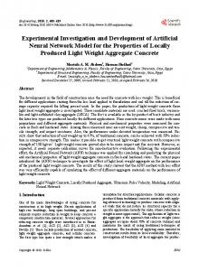
about the underlying relationships. These non linear models can approximate unknown mappings and its derivatives by a three-layer structure: input, hidden and output layers (Hornik et al. 1989; 1990). The common networks are the feedforward neural networks or multilayer perceptron, where the connections between the neurons are from the input to the output without feedbacks. The architecture selection and the neural learning are basic issues in the neural modelling. In the architecture selection, or model selection in econometric language, the researcher must determine the number of input and hidden units and the activation function. A data preprocessing can also be applied (e.g., [0,1]). The lack of a general procedure results in a trial and error process, and the final architecture is selected according to some information criterion (AIC or SIC). A multilayer perceptron can be expressed as: q y = f ( x, θ ) + ε = β 0 + ∑ j =1 β j G( x~ ′γ j ) + ε (1) where ~x = (1, x1 , x 2 ,..., x r )′ , j = 1, ..., q; θ = ( β0 , β1 ,..., βq , γ 1′ ,..., γ ′q ) . Figure 1. A three-layer neural network ∑ (β) 1

∑

∑

(γ) 1 X1

X2

X3

...

Xr

The transfer function is usually chosen to be monotone and nondecreasing. In this paper the output activation function is linear, and the hidden transfer function (G) is logistic or hyperbolic tangent. The logistic function maps into the [0,1] interval, whereas the tanh maps into the [-1,1] rank. In the training phase, estimation in econometric jargon, the backpropagation algorithm (Rumelhart et al., 1986) is the most used method. BP is a gradient (steepest) descent method that minimizes an error function (sum of error squares) by modifying the network parameters according to: θ k +1 = θ k + η

∂E ∂θ k

(2)

where k denotes the iteration number, and η the learning rate between 0 and 1. However, the BP has been severely criticized and new alternatives were further analysed. On this topic, the Levenberg-Marquardt algorithm can improve significantly the performance of BP (Hagan and Menhaj, 1994).

2

3. Methodologies In this section we briefly review the three methodological approaches to efficiency measurement: parametric techniques, non-parametric techniques and artificial neural networks. A complete description of these techniques can be found in Kumbhakar and Lovell (2000) and a recent survey is available in Murillo-Zamorano (2004). The parametric approach to estimate technical efficiency indexes requires the specification of a functional form for the production frontier, i.e. a production function, with the risk of functional form mis-specification. Although the simple Cobb-Douglas specification has been the most widely used functional form, other functions such as the translog, CES or generalized Leontief allow for more flexibility and, thus, provide a better adjustment to the actual data. Two different efficiency models can be found within the parametric literature. The first to be used was the deterministic frontier, where any deviation from the data to the frontier (i.e. error terms) was attributed to inefficiency (Aigner and Chu, 1968). In contrast, stochastic frontier models allow for a decomposition of the error term into a symmetric part that is interpreted as random error and a non-symmetric part that is interpreted as technical inefficiency (Aigner et al., 1977). The non-parametric approach makes no assumption about the functional form of the frontier. Instead, it specifies certain assumptions about the underlying technology that in combination with the data set allow the construction of the production set. The non parametric approach is usually referred to as the DEA approach (i.e., Data Envelopment Analysis) since the seminal paper of Charnes et al. (1978) who assumed a technology satisfying constant returns to scale (CRS), convexity, and free disposability of inputs and outputs. The efficiency index is estimated by solving a mathematical program that finds the maximum increase in the outputs or reduction in the inputs combining the information about production practices actually observed in the data set with the assumptions made for the technology. The program compares the input-output vector of the firm which efficiency is being measured with the composite virtual firm (constructed from the data and the technological assumptions made) that uses the same inputs to produce the largest possible output or produces the same quantity of the output but using the lowest possible quantities of inputs. The DEA(CRS) approach has been subject to continuous modifications aimed to relax some of its assumptions or to change the orientation of the efficiency index estimated. The most notable changes are known as the DEA(VRS) and the FDH approaches. DEA(VRS) simply relaxes the assumption of constant returns to scale (Banker et al. 1984), by restricting the production set to the convex combinations of the production vectors of the firms actually sampled. The FDH (Free Disposal Hull) technique goes a step further by dropping the convexity assumption. The production set is then constructed from the sample data and the assumption of free disposability, but does not allow for the use of composite (convex) virtual units (Deprins et al., 1984; Tulkens, 1993). Note that the inneficient units under FDH are marked as inneficient units in DEA too, but the opposite is not true. One major limitation of FDH approach is the considerable number of efficient units. Finally, in the neural network approach we may consider three alternatives: §

From the estimated network - ANN1.

3

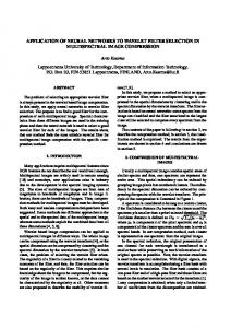
In this approach the efficiency measure of a unit is established in relation to the average performance. Thus, the indicators will be superior to 1 or 100% when the unit behaves better than average, and inferior to 1 or 100% if the unit is “inefficient”. These measures are not directly comparable with the traditional techniques. Athnassopoulos and Curram (1996) called this option “non-standarized efficiency” ENE: y E NE = i (3) i yˆ i To achieve a real production frontier there are some alternatives: § Shift the network by the largest positive error – ANN2. This option is similar to COLS. The correction by the largest positive error is sensitive to outliers and the frontier will be deterministic. The efficiency scores take values between 0 and 1. This maximum score is assigned to the unit used for the correction. Athnassopoulos and Curram (1996) called this second measure “standarized efficiency” EE: yi E Ei = (4) yˆ i + max i εˆ i In relation to DEA, the non-standarized efficiency (ENE) tends to overestimate the indicators, and the standarized efficiency (EE) tends to underestimate the measures. § Shift the network by a mean of the largest positive errors – ANN3. For attenuating the effect of the largest positive error, in this work a new approach is proposed. This option consists of not considering the largest, but some percentage (5 per cent) of the largest positive errors: E ′i E =

yi

(5)

yˆ i + avg (εˆi5 % )

Figure 2. Production function and frontier function from neural network Y Frontier ANN2

• •

extreme

•

• •

•

• • maximum • •

• Frontier ANN3

average

•

•

•

• •

•

•

Production ANN1

•

•

X

To conclude this section, a rough comparison of the three methodological approaches (parametric, non parametric and neural network) is given in Table 1. In summary, the neural network approach requires no assumptions about the production function (the major drawback of the parametric approach) and it is highly flexible. Nevertheless, future research with neural networks in the efficiency analysis is required.

4

Table 1. Comparison of the methodological approaches to efficiency measurement Comparative Factor Parametric Non Neural parametric network Assumptions: functional form, data Strong Medium Low Flexibility Low-Medium Medium High Theoretical studies/applications on efficiency Yes Yes Few Costs: software, estimation time Low Low High Efficiency measure compares the observed A specific A piecewise A non linear unit with the frontier... functional linear function with form envelopment minimum assumptions

4. Data and results For illustrating the potential of the artificial neural networks, a comparative study is carried out in the public sector context, specifically the refuse collection services (Bosch et al., 2000) from a sample of 72 spanish municipalities. The output considered is the solid waste (SOW) and the inputs include the containers capacity (CON), vehicles (VEH) and worked hours (WOR). The summary statistics are presented in the Table 2.

Minimum Maximum Mean Standard deviation Variation coefficient 1st quartile Median 3rd quartile Correlation Output RES Input 1 CON Input 2 VEH Input 3 WOR

Table 2. Summary statistics Output SOW Input 1 CON Input 2 VEH Input 3WOR 1506.20 67.20 4.00 480.00 88309.00 5279.15 329.00 420480.00 13321.62 655.47 49.53 24088.50 18015.36 970.33 61.82 52709.46 1.35 1.48 1.25 2.19 3799.39 7389.00 13167.70

181.16 360.15 642.83

18.88 26.50 50.00

5515.00 8845.50 19514.70

1.000 0.931 0.929 0.487

1.000 0.817 0.419

1.000 0.504

1.000

In the parametric context, a Cobb-Douglas function and a translog function were estimated. Nevertheless, the differences between them were negligible and we selected the CobbDouglas because of simplicity (Table 3). The correlation between the inputs 1 and 2 causes a non significative parameter for the latter, but this may no affect the estimation of the efficiency scores.

5

Constant Ln CON Ln VEH Ln WOR λ=σu/σv (u semi-normal) σ=(σ2 u+σ2 v )1/2 Adjusted R2 Scale returns Wald´s test Hypot: β1 +β2 +β3 =1

Table 3. Cobb-Douglas results Cobb-Douglas det. Cobb-Douglas stoc. 2.2188 (7.17) 2.3240 (3.21) 0.8002 (13.20) 0.8004 (12.77) -0.0483 (-0.67) -0.0494 (-0.73) 0.2311 (4.58) 0.2321 (3.965) 0.5286 (0.17) 0.2996 (1.26) 0.9176 F=0.1797 p=0.673

The estimated neural network incorporates four tanh hidden units and the LevenbergMarquardt algorithm is employed for the training (Table 4). Table 4. Estimated neural network Concept Result Data pre-processing [-1,1] Network architecture 3-4-1 Activation function: hidden / output tanh / linear Algorithm Levenberg-Marquardt Epochs (max.) 1000 R2 0,9854 The main results are summarized in the Table 51 . Several differences are clearly appreciated. First, all methodologies assign 1 to the most efficient unit appart from the stochastic CobbDouglas and ANN1. Stochastic Cobb-Douglas and FDH show higher mean scores, and the ANNs models show the highest standard deviations. Finally, the number of efficient units is different from one approach to the other. Under FDH, most units, 45 of 72, are efficient, whereas the deterministic Cobb-Douglas and ANN2 indicate only one efficient unit.

Mean Minimum Maximum Rank 1st quartile Median 3rd quartile Stand deviat Variat. Coef. Effic. units

1

Table 5. Efficiency main results C-Ddet C-Dsto DEAcrs DEAvrs FDH 0.5227 0.8946 0.6049 0.7268 0.9145 0.2698 0.8318 0.2796 0.3277 0.4672 1.0000 0.9374 1.0000 1.0000 1.0000 0.7302 0.1056 0.7204 0.6723 0.5328 0.4339 0.8847 0.4987 0.5979 0.8534 0.5103 0.8986 0.5651 0.6957 1.0000 0.5959 0.9100 0.7285 0.8901 1.0000 0.1483 0.0232 0.1882 0.1918 0.1367 0.2837 0.0260 0.3111 0.2639 0.1495 1 0 7 15 45

Detailed results are available from the author upon request.

6

ANN1 1.0118 0.5092 1.8640 1.3548 0.8751 1.0000 1.1173 0.2698 0.2666 35

ANN2 0.5221 0.1671 1.0000 0.8329 0.3101 0.4944 0.7004 0.2365 0.4530 1

ANN3 0.5569 0.1903 1.0000 0.8097 0.3383 0.5374 0.7391 0.2360 0.4238 2

In this analysis a key objective consists of showing if there exist differences in the ranking. A correlation study is carried out and the Pearson´s coefficient (Table 6) and the Spearman´s rank coefficient (Table 7) are shown. From the Table 6, the ANN1 results are highly correlated with those obtained in the parametric (0.8) and DEAcrs (0.7) techniques. The ANN2 and ANN3 models show correlations about 0.5 with the same methods, and the non parametric models present similar results. The same conclusions can be reached from the results reported in Table 7. Again, the neural models 2 and 3 performance is different and provide alternative results from the traditional approaches. Finally, all methodologies agree with the most efficient units and those municipalities with the lowest scores, so these results are more robust. Table 6. Pearson´s correlation coefficient C-Ddet C-Dsto DEAcrs DEAvrs FDH ANN1 ANN2 ANN3

C-Ddet C-Dsto DEAcrs DEAvrs FDH 1 0.9373 1 0.7716 0.7617 1 0.6413 0.6550 0.7861 1 0.5099 0.6025 0.5871 0.7411 1 0.8221 0.7829 0.7015 0.5962 0.5638 0.5269 0.4694 0.4380 0.3750 0.2628* 0.5478 0.4917 0.4576 0.3764 0.2751*

ANN1

ANN2

ANN3

1 0.4173 0.4437

1 0.9986

1

ANN2

ANN3

1 0.9986

1

All coefficients are significative at 1% level, except * , at 5%

C-Ddet C-Dsto DEAcrs DEAvrs FDH ANN1 ANN2 ANN3

Table 7. Spearman´s rank-correlation coefficient C-Ddet C-Dsto DEAcrs DEAvrs FDH ANN1 1 0.9999 1 0.8326 0.8343 1 0.6368 0.6385 0.7626 1 0.5359 0.5359 0.6451 0.7964 1 0.7841 0.7846 0.7812 0.5996 0.6041 1 ** 0.4694 0.4689 0.4877 0.3076 0.2281 0.3940 * 0.4909 0.4904 0.5094 0.3229 0.2485 0.4208

All coefficients are significative at 1% level, except * , at 5%, and ** , at 10%

5. Concluding remark Today, several approaches for the efficiency measurement are available. The parametric techniques, both deterministic and stochastic, and non parametric approaches, like DEA and FDH, are the most widely-used. In this paper we have used the ANNs to measure and rank the decision-making units efficiency because the neural networks, universal aproximators of functions and its derivates, are non linear and highly flexible models.

7

The application to the refuse collection services shows that the neural networks offer new insights into the efficiency analysis. Although several differences in the quantitative measures are evidenced, it is important to note that there exist common trends as shown by the correlation and rank-correlation analysis. The most efficient units were identified by practically all the approaches, and also the lowest efficient units, so these results are more robust. As a final remark, we believe it is useful to view the neural networks as a complementary, rather than alternative, tool for efficiency analysis.

References Aigner, D.J. and S.F. Chu (1968) “On Estimating the Industry Production Function” American Economic Review 58(4), 826-839. Aigner, D.J., C.A.K. Lovell and P. Schmidt (1977) “Formulation and estimation of stochastic frontier production function models” Journal of Econometrics 6, 21-37. Athnassopoulos, A. and S. Curram (1996) “A comparison of data envelopment analysis and artificial neural networks as tools for assessing the efficiency of decision-making units” Journal of the Operational Research Society 47, 1000-1016. Banker, R.D., A. Charnes and W. Cooper (1984) “Some models for the estimation of technical and scale efficiencies in data envelopment analysis” Management Science 30(9), 1078-1092. Charnes A, W. W. Cooper and E. Rhodes (1978) “Measuring the efficiency of decision making units” European Journal of Operational Research 2, 429-444. Costa, A. and R.N. Markellos (1997) “Evaluating public transport efficiency with neural network models” Transportation Research C 5(5), 301-312. Deprins, D., L. Simar and H. Tulkens (1984) “Measuring labour-efficiency in post offices” in The performance of public enterprises: concepts and measurements by M. Marchand, P. Pestieau and H. Tulkens, Eds, North-Holland: Amsterdam, 243-267. Farrell, M.J. (1957) “The measurement of productive efficiency” Journal of the Royal Statistical Society 120, 253-281. Fleissig, A.R., T. Kastens and D. Terrell (2000) “Evaluating the semi-nonparametric fourier, aim, and neural networks cost functions” Economics Letters 68(3), 235-244. Fox, K.J., Ed. (2002) Efficiency in the Public Sector, Kluwer Academic Publishers: Massachusetts. Hagan, M.T. and M. Menhaj (1994) “Training feedforward networks with the marquardt algorithm” IEEE Transactions on Neural Networks 5(6), 989–993. Hornik, K., M. Stinchcombe and H. White (1989) “Multilayer feedforward networks are universal approximators” Neural Networks 2, 359-366. Hornik, K., M. Stinchcombe and H. White (1990) “Universal approximation of an unknown mapping and its derivatives using multilayer feedforward networks” Neural Networks 3, 551-560. Joerding, W, Y. Li, S. Hu and J. Meador (1994) “Approximating production technologies with feedforward neural networks” in Advances in artificial intelligence in Economics, Finance and Management 1 by J.D. Johnson and A.B. Whinston, Eds, JAI Press: London, 35-42. 8

Kumbhakar, S.C. and C.A.K. Lovell (2000) Stochastic frontier analysis, Cambridge University Press: Cambridge. Murillo-Zamorano, L. (2004) “Economic efficiency and frontier techniques” Journal of Economic Surveys 18(1), 33-77. Rumelhart, D., G. Hinton and R. Williams (1986) “Learning internal representations by error propagation” in Parallel distributed processing: explorations in the microstructures of cognition 1 by D. Rumelhart and J. McClelland, Eds, MIT Press: Cambridge, 318-362. Santín, D., F.J. Delgado and A. Valiño (2004) “The measurement of technical efficiency: a neural network approach” Applied Economics 36(6), 627-635. Tulkens, H. (1993) “On FDH analysis: some methodological issues and applications to retail banking, courts and urban transit” Journal of Productivity Analysis 4, 183-210. Vellido, A., P.J.G. Lisboa and J. Vaughan (1999) “Neural networks in business: a survey of applications (1992–1998)” Expert Systems with Applications 17, 51–70.

9