Memory Architecture Impact on FPGA Energy ... - Semantic Scholar

Impact of Memory Architecture on FPGA Energy Consumption Edin Kadric David Lakata [email protected] [email protected]

André DeHon [email protected]

Department of Electrical and Systems Engineering University of Pennsylvania 200 S. 33rd St., Philadelphia, PA 19104

ABSTRACT FPGAs have the advantage that a single component can be configured post-fabrication to implement almost any computation. However, designing a one-size-fits-all memory architecture causes an inherent mismatch between the needs of the application and the memory sizes and placement on the architecture. Nonetheless, we show that an energybalanced design for FPGA memory architecture (memory block size(s), memory banking, and spacing between memory banks) can guarantee that the energy is always within a factor of 2 of the optimally-matched architecture. On a combination of the VTR 7 benchmarks and a set of tunable benchmarks, we show that an architecture with internallybanked 8Kb and 256Kb memory blocks has a 31% worstcase energy overhead (8% geomean). In contrast, monolithic 16Kb memories (comparable to 18Kb and 20Kb memories used in commercial FPGAs) have a 147% worst-case energy overhead (24% geomean). Furthermore, on benchmarks where we can tune the parallelism in the implementation to improve energy (FFT, Matrix-Multiply, GMM, Sort, Window Filter), we show that we can reduce the energy overhead by another 13% (25% for the geomean).

Categories and Subject Descriptors B.7.1 [Integrated Circuits]: Types and Design Styles

Keywords FPGA, Energy, Power, Memory, Architecture, Banking

1.

INTRODUCTION

Energy consumption is a key design limiter in many of today’s systems. Mobile devices must make the most of limited energy storage in batteries. Limits on voltage scaling mean that even wired systems are often limited by power density. Reducing energy per operation can increase the performance delivered within a limited power envelope. Permission to make digital or hard copies of all or part of this work for personal or classroom use is granted without fee provided that copies are not made or distributed for profit or commercial advantage and that copies bear this notice and the full citation on the first page. Copyrights for components of this work owned by others than ACM must be honored. Abstracting with credit is permitted. To copy otherwise, or republish, to post on servers or to redistribute to lists, requires prior specific permission and/or a fee. Request permissions from [email protected]. FPGA’15, February 22–24, 2015, Monterey, California, USA. Copyright is held by the owner/author(s). Publication rights licensed to ACM. ACM 978-1-4503-3315-3/15/02 ...$15.00. http://dx.doi.org/10.1145/2684746.2689062.

Memory energy can be a significant energy component in computing systems, including FPGAs. This is particularly true when we assess the total cost of memories, including interconnect energy on wire segments that carry data to distant and distributed memory blocks or to off-chip memory. This leads to an important architectural question: How do we organize memories in FPGAs to minimize the energy required for a computation? We have several choices: What are the sizes of memory blocks? Where (how frequently) are memory blocks placed in the FPGA? How are they activated? How are they decomposed into sub-block banks? Then, there are choices available to the RTL mapping flow: When mapping a logical memory to multiple blocks, should they each get a subset of the data width and be activated simultaneously? or should they each get a subset of the address range and be activated exclusively? In this paper, we first develop simple analytic relations to reason about these choices (Section 2). After reviewing some background in Section 3, we describe our methodology in Section 4. In Section 5, we perform an empirical, benchmark-based exploration to identify the most energy-efficient organization for memories in FPGAs and quantify the trade-offs between area- and energy-optimized mappings. Section 6 takes the study from Section 5 one step further. For high-level tasks, we are not stuck with a single memory organization—the choice of parallelism in the design impacts the memory organization needed and, consequently, the total energy for the computation. A highly serial design might build a single processing element (PE) and store data in a single large memory; whereas a more parallel version would use multiple PEs and multiple, smaller memory blocks. The parallel version would then have lower memory energy, but may spend more energy on routing. Consequently, there is additional leverage to improve energy by selecting the appropriate level of parallelism. In Section 6, we explore how this selection allows energy savings and how it further drives the selection of energy-efficient FPGA memory architectures. Contributions: • Analytic characterization of the energy overhead that results from mismatches between the logical memory organization needed by a task and the physical memory organization provided by an FPGA (Section 2) • First empirical exploration of memory architecture space for energy minimization (Section 5) • VTR-compatible memory mapping for energy minimization (Section 4.2) • Joint exploration of memory architecture space and high-level parallelism tuning (Section 6)

Therefore:

dm=4

&r Emseg (March )

LB Memory

Block

Mapp March

' ≈ Emseg (Mapp ) ≈ 0.5Ebit (Mapp )

This gives us the following mismatch ratio, driven by the ratio of the energy for routing between memory banks to the energy for routing over memory banks: Lmseg

Lseg

dm Eseg Eh + Ev ≈1+ Ebit (Mapp ) 2Emseg (March )

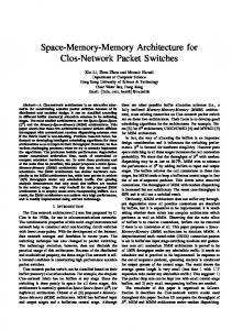
Figure 1: Column-Oriented Embedded Memories

2.

ARCHITECTURE MISMATCH ENERGY

FPGA embedded memories generally improve area- and energy-efficiency [10]. When it perfectly matches the size and organization needed by the application, an FPGA embedded memory can be as energy-efficient as the same memory in a custom ASIC. Nonetheless, the FPGA has a fixedsize memory that is often mismatched with the task, and this mismatch can be a source of energy overhead. First, let us consider just the memory itself. Memory energy arises almost directly from the energy to charge wire capacitance, which grows as the side length of the memory; that is, in an energy-minimizing layout, a memory block will roughly be square and the length of address lines, bit lines, and output wires grow as the square root of the memory capacity. A memory that is four times as large will require twice the energy. Therefore, when the FPGA memory block (March ) is larger than the application memory (Mapp ), there is an energy overhead that arises directly from reading from a memory bank that is too large (E(March )/E(Mapp )). There is also a mismatch overhead when the memory block is smaller than the application memory. To understand this, we must also consider the routing segments needed to link up the smaller memory banks into a larger memory bank. To build a larger bank, we take a number of memory banks (dMapp /March e) and wire them together, with some additional logic, to behave as the desired application memory block. In modern FPGAs it is common to arrange the memory blocks into periodic columns within the FPGA logic fabric (See Fig. 1). Assuming square memory and logic blocks, the set of smaller memory blocks used to realize the large memory block m be organized into a square of lpwould roughly Mapp /March , demanding that each address side length bit and to the memory cross roughly lpdata line connected m dm × Mapp /March horizontal interconnect segments to address the memory, where dm is the distance between memory columns in the FPGA architecture. If Eseg is the energy to cross a length-1 segment over a logic island in the FPGA and Emseg (March ) is the energy to cross a length-1 segment over a memory block of capacity March , the horizontal and vertical routing energy to reach across the memory is: m lp Mapp /March (1) Eh = (dm Eseg + Emseg (March )) × Ev = Emseg (March )

lp m Mapp /March

(2)

Since the routing energy of wires comprises most of the energy in a memory read, and since each bit must travel the height of the memory block (bit lines) and the width (output select), per bit, the energy of a memory read is roughly the energy of the wires crossing it: Ebit (M ) ≈ 2Emseg (M )

(3)

(4)

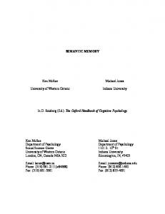
To illustrate the mismatch effects, Fig. 3a shows the result of an experiment where we quantify how the energy compares between various matched and mismatched designs. Each of the curves represents a single-processing-element matrix-multiply design that uses a single memory size; the size of the memory varies with the size of the matrices being multiplied. Each curve shows the energy mismatch ratio (Yaxis) between the energy required on a particular memory block size (X-axis) and the energy required at the energyminimizing block size (typically the matched size); hence all curves go to 1.0 at one memory block size and increase away from that point. In contrast to the previous paragraph where we used deliberately simplified approximations to provide intuition, Fig. 3a is based on energy from placedand-routed designs using tools and models detailed in the following sections; Fig. 3 also makes no a priori assumption about large memory mapping, allowing VTR [15] to place memories to minimize wiring. The figure shows how the energy mismatch ratio grows when the memory block size is larger or smaller than the matched memory block size. In practice, designs typically demand a mix of memory sizes, making it even harder to pick a single size that is good for all the memory needs of an application. Nonetheless, this single-memory size experiment is useful in understanding how each of the mismatched memories will contribute to the total memory energy overhead in a heterogeneous memory application. There is also a potential energy overhead due to a mismatch in memory placement. Assuming we accept a columnoriented memory model, this can be stated as a mismatch between the appropriate spacing of memories for the application (dmapp ) and the spacing provided by the architecture (dmarch ). If the memories are too frequent, non-memory routes may become longer due to the need to route over unused memories. If the memories are not placed frequently enough, the logic may need to be spread out, effectively forcing routes to be longer as they run over unused logic clusters. This gives rise to a mismatch ratio: m ld mapp (dmarch Eseg + Emseg (March )) dmarch (5) dmapp Eseg + Emseg (March ) Note that if we make dmarch Eseg = Emseg (March ), the mismatch ratio due to route mismatch (Eq. 5) is never greater than 2×. Similarly, the mismatch ratio due to memories being too small (Eq. 4) is never greater than 1.5×. We can observe this phenomenon in Fig. 3a by looking at the 32Kb memory size that never has an overhead greater than 1.2×. In Fig. 3, we also identify the dmarch that minimizes maxoverhead (shown between square brackets for each memory size in Fig. 3). This approximately corresponds to the intuitive explanation above, where the energy for routing across memories is balanced with the energy for routing across

(a) Normal Memories

Lmseg(M)

● ●

32 64 128 256 512

●

● ● ● ●

● ● ●

0.5 [1]

1 [1]

●

2 [1]

Data

Figure 2: Internal Banking of Memory Block

0.5 1 2 4 8 16

●

1

Lmseg(M) Lmseg(M/4)

Addr[n-1] Addr[n-3:0] Addr[n-2]

Normalized Total Energy 2 3

App Mem Size (Kb)

Lmseg(M/4)

●

●

●

●

●

●

●

●

●

4 8 16 32 64 128 256 512 [1] [1] [2] [2] [3] [3] [7] [7] Physical Memory Size (Kb) [dm]

(b) Memories with Internal Banking (one quarter, one sixteenth)

Normalized Total Energy 2 3

App Mem Size (Kb) ● ●

0.5 1 2 4 8 16

32 64 128 256 512

●

●

● ● ●

1

logic. The 32Kb case has Emseg (March )/Eseg = 2.53, suggesting a dmarch of 2 or 3. For this 32Kb case, we found dmarch = 2 experimentally. Since segment energy is driven by wire length, dmarch Eseg = Emseg (March ) roughly means dmarch Lseg = Lmseg (March ); when we populate memories this way, half the FPGA area is in memory blocks. This design point gives us an energy-balanced FPGA that makes no a priori assumptions about the mix of logic and memory in the design. In contrast, today’s typical commercial FPGAs could be considered logic-rich, making sure the energy (and area) impact of added memories is small on designs that do not use memories heavily. While the dmarch Eseg = Emseg (March ) balance can limit the overhead when the memories are too small, we can still have large overhead when the memory blocks are too large (E(March )/E(Mapp )). One way to combat this problem is to use internal banking, or Continuous Hierarchy Memories (CHM) [8]: We can bank the memory blocks internally so that we do not pay for the full cost of a large memory block when we only need a small one. For example, if we cut the memory block into four, quarter-sized memory banks, and only use the memory bank closest to the routing fabric when the application only uses one fourth (or less) of the memory capacity, we only pay the memory energy of the smaller memory bank (See Fig. 2). In the extreme, we might recursively decompose the memory by powers-of-two so that we are never required to use a memory more than twice the size of the memory demanded by the application. There are some overheads for this banking which may suggest stopping short of this extreme. Fig. 3b performs the same experiment as Fig. 3a, except with memory blocks that can be decomposed into one-quarter and one-sixteenth capacity sub-banks. With this optimization, the curves flatten out for larger memory sizes. The physical size with smallest max-overhead is now shifted to 128Kb, still at 1.2×. Another way to reduce the impact of memory block size mismatch is to include memory blocks of multiple sizes in the architecture. This way, the design can use the smallest memory block that will support the application memory. For example, if we had both 1Kb and 64Kb memories, we could map the 2Kb and smaller application memories to the 1Kb memory block and the 4Kb and larger application memories to the 64Kb block and reduce the worst-case overhead to 1.1× (Fig. 3a). However, this raises an even bigger question

●

0.5 [1]

●

1 [1]

●

2 [1]

●

●

●

● ●

● ●

● ●

●

● ●

4 8 16 32 64 128 256 512 [1] [1] [2] [2] [3] [3] [7] [7] Physical Memory Size (Kb) [dm]

Figure 3: Energy Overhead due to Architectural Mismatch for Matrix-Multiply about balance among logic and the multiple memory sizes. In particular, routes may now need to pass over the memory blocks of the unused size. We can generalize the previous observation about balancing routing over memories and logic to: dm1 Eseg = Emseg (M1 ), dm2 Eseg = Emseg (M2 ). However, since there are now three different resource types, in the worst-case, a route could need 3× the energy of the optimally-matched architecture instead of 2× when there were only two resource types (logic and one memory size). Another point of mismatch between architecture and application is the width of the data read or written from the memory block. Memory energy also scales with the datawidth. In particular, energizing twice as many bit lines costs roughly twice the energy. While FPGA memory blocks can be configured to supply less data than the maximum width, this is typically implemented by multiplexing the wider data down to smaller data after reading the full width—the same number of bit lines are energized as the maximum width case, so these smaller data reads are just as expensive as the maximum width read, and hence more expensive than they could have been with an optimally-configured memory. While width mismatch is another, important source of mismatch, it is beyond the scope of this paper. We stick to a single raw data-width of 32 bits throughout our experiments. Another potential point of mismatch is the simultaneous ports provided by the memories. We assume all memories are dual-ported (2 read/write ports) throughout this paper.

3.

FPGA Memory Architecture

We build on the standard Island-Style FPGA model [3]. The basic logic tile is a cluster of K-LUTs with a local crossbar providing connectivity within the cluster (c.f. Xilinx CLB, Altera LAB). These clusters are arranged in a regular mesh and connected by segmented routing channels. To incorporate memories into this mesh, we follow the model used by VTR [15], Xilinx, and Altera, where select columns are designated as memory columns rather than logic columns (Fig. 1). Organizing the memory tiles into a homogeneous column rather than placing them more freely in the mesh allows them the freedom to have a different size than the logic tiles. For example, if the memory block requires more area than the logic cluster, we can make the memory column wider without creating irregularity within rows or columns. Altera uses this column memory model in their Cyclone and Stratix architectures, and the M9K blocks in the Stratix III [12] are roughly 3× the area of the logic clusters (LABs) [20], while being logically organized in the mesh as a single tile. Large memories can span multiple rows, such as the M144K blocks in the Stratix III, which are 8-rows tall while remaining one logical row wide, accommodated by making the column wider as detailed above. Within this architectural framework, we can vary the proportion of memory tiles to logic tiles by selecting the fraction of columns that are assigned to memory tiles rather than logic tiles. One way to characterize this is to set the number of logic columns between memory columns, dm . VTR identifies this as a repeat parameter (repeat=dm + 1). For two memory sizes, dm still gives the spacing between memory columns, but we first use h1 /h0 memory columns with small memories of height h0 , followed by one column of large memories of height h1 , so that the area occupied by the small memories is equal to the area occupied by the large ones.

3.2

Energy Modeling and Optimization

Poon [17] developed energy modeling for FPGAs and identified how to size LUTs (4-LUTs), clusters (8–10), and segments (length 1) to minimize energy. However, Poon did not identify an energy-minimizing memory organization. FPGA energy modeling has since been expanded to modern directdrive architectures and integrated into VTR [6]. Recent work on memory architecture has focused on area optimization rather than energy. Luu examined the areaefficiency of memory packing and concluded that it was valuable to support two different memory block sizes in FPGAs [14]. Lewis showed how to size memories for area optimization in the Stratix V and concluded that a single 20Kb memory was superior to the combination of 9Kb and 144Kb memories in previous Stratix architectures [13], but did not address energy consumption, leaving open the question of whether energy-optimized memory architectures would be different from area-optimized ones.

3.3

Memory Energy Modeling

We use CACTI 6.5 [16] to model the physical parameters (area, energy, delay) of memories as a function of capacity, organization, and technology. In addition to modeling capacity and datapath width, CACTI explores internal implementation parameters to perform trade-offs among area, delay, throughput, and power. We use it to supply the mem-

58

Addresses 0–63 64–255 256–1023 Shape 16×32 48×32 192×32 Size (µm2 ) 38×15 52×31 94×58 Emem (pJ) 0.31 0.54 1.1 Ewires (pJ) 0.0 0.46 0.84

15 64 x 38 32

94

768x32

(in μm)

192 x32

52

31

Figure 4: Internal Banking for 32K memory Verilog p-opt

CACTI ITRS VTR Odin

Arch Blif simulation Activity ABC

VPR

Energy

Figure 5: Energy Estimation Tool Flow ory block characteristics for VTR architecture files at 22 nm. We set it to optimize for the energy-delay-squared product. For internal banking (Fig. 2), CACTI gives us the area and energy (Emem ) of the memory banks, and we compute wire signaling energy (Ewires ) to communicate data and addresses between the referenced memory bank and the memory block I/O. For example, consider the data in Fig. 4 for a 1024×32b (32Kb) internally-banked memory. A monolithic 32Kb memory block is 67µm×113µm, which is high enough to contain the 94µm required for the height of the 768 × 32 memory of size 58µm×94µm (plus room for extra logic), as shown in Fig. 4. The total width in Fig. 4 is 58 + 31 = 89µm, or 89/67 = 1.33× that of the monolithic 32Kb memory block. We therefore adjust Emseg (32K-banked)= 1.33 × Emseg (32K). CACTI directly provides Emem . For the largest bank, Ewires is (31µm)(1 + 10 + 64)Cwire (Vdd )2 . Cwire = 180pF/m, Vdd = 0.95V. (1 + 10 + 64) corresponds to one signal for the enable, 10 for the address bits, 64 for the 32b input and 32b output. 31µm is the distance to reach the large bank. The medium-size bank has a similar Ewires equation but with 38µm instead of 31µm, and the small bank has Ewires = 0. Then, the energy of an internally-banked memory is given by Ebanked = Emem + αEwires , where α is the average activity factor over all signaling wires.

4.

METHODOLOGY

Fig. 5 shows our tool flow. We developed and added several components on top of a stock VTR 7 release.

4.1

Activity Factor Simulation

Activity factors and static probabilities assigned to the nets of a design have a major impact on the estimated energy. Common ways to estimate activity include assigning a uniform activity to all nets (e.g., 15%), or performing vectorless estimation with tools such as ACE [11], as done by VTR. For better accuracy, our flow obtains activity factors by simulating the designs. We run a logic simulation on the BLIF output of ABC (pre-vpr.blif file) on a uniformly random input dataset. For example, for the matched 32Kbmemory matrix-multiply design in Fig. 3a, the average simulated activity factor is 11%, whereas ACE estimates it to be 3%, resulting in an energy estimation that is off by ≈ 3.7×. The tunable benchmarks are designed in a streaming way that activates all memories all the time (independent of the random data), except Matrix Multiply (MMul), for which the clock-enable signal is on ≈ 1/3 of the time. The VTR benchmarks do not come with clock-enable for the memories, so we set them to be always on.

I/O

3.1

BACKGROUND

addr

8K 8K 8K 8K [10:8] 8K 8K 8K 8K 32b

4b 4b 4b 4b en en en en

4.4

12 8 4 0

4 8 16 32

0 en

addr[10:0] en en en en

Energy (pJ)

addr[7:0]

W logic 8K 8K 8K 8K route 4b 4b 4b 4b mem a: 2K×32 (W=32) b: 2K×32 (W=4) c: Sweep W Figure 6: Effect of Memory Block Activation and Output Width Selection on Energy Consumption

8K 8K 8K 8K

4.2

Power-Optimized Memory Mapping

When mapping logical memories onto physical memories, FPGA tools can often choose to optimize for either delay or energy using power-aware memory balancing [19]. For example, when implementing a 2K×32b logical memory using eight 256×32b physical memories, the tool could choose to read W = 4b from each memory (delay-optimized, Fig. 6b). Since each memory internally reads at the full, native width, the cost of the memory operation is multiplied by the number of memory blocks used. Alternatively, it could read W = 32b from only one of the memories (Fig. 6a), in which case only one memory is activated at a time (reducing memory energy), but extra logic and routing overhead is added to select the appropriate memory and data. The poweroptimized case often lies between these extremes. For example, as our experiment shows in Fig. 6c, the optimum is to activate 2 memories at once and read W = 16b from each. Unfortunately, the VTR flow does not perform this kind of trade-off: it always optimizes for delay. Odin decomposes the memories into individual output bits [18], and the packer packs together these 1-bit slices as much as possible within the memory blocks to achieve the intended width [14]. In fact, VTR memories do not have a clock-enable so they must be activated all the time. Instead, we use VTR architectures with special memory block instantiations that contain a clock-enable, modify VTR’s architecture-generation script (arch_gen.py) to support these blocks and to support two memory sizes, and add a p-opt stage before Odin to perform power-optimized memory mapping based on the memories available in the architecture. This includes performing memory sweeps as illustrated in Fig. 6c to select the appropriate mapping for each application memory. The impact of this optimization is shown for the best architectures in Tab. 2. We find that mapping without p-opt adds 4-19% geomean energy overhead for the optimum architectures, comparable to the 6% benefit reported in [19]. Not using p-opt adds 40–108% worst-case energy overhead, suggesting that this optimization is more important for the designs with high memory overhead. Our p-opt code and associated VTR architecture generation script can be found online [7].

4.3

Logic Architecture

The logic architecture uses k4n10 logic blocks (clusters of 10 4-LUTs) and 36×36 embedded multipliers (which can be decomposed into two 18×18 multiplies, or four 9×9 multiplies) with dmpy =10 and the same shape and energy as in VTR’s default 22 nm architectures (a height of 4 logic tiles, plus we use Lmpyseg = 4Lseg ). The routing architecture uses direct-drive segments of length 1 with Wilton switch-boxes.

Technology

We use Low Power (LP) 22 nm technology [1] for logic evaluation and Low Stand-by Power (LSTP) for memories. We use ITRS parameters for constants such as the unit capacitance of a wire at 22 nm (Cwire = 180 pF/m). Then: Cmetal = Cwire × tile-length (6) We evaluate interconnect energy based on this Cmetal , instead of the constant one that is provided in the architecture file. This way, the actual size of the low-level components of the given architecture and technology, as well as the computed channel width, are taken into account when evaluating energy. It is important to model this accurately since routing energy dominates total FPGA energy (See Fig. 6c).

4.5

Energy and Area of Memory Blocks

VTR assigns one type of block to each column on the FPGA (logic cluster, multiplier, or memory), and can give them different heights, but assumes the same horizontal segment length crossing each column. However, some memories can occupy a much larger area than a logic tile, and laying them out vertically to fit in one logic tile width would be inefficient. For energy efficiency, the memories should be closer to a square shape, and to that end, we allow the horizontal segment length crossing memories to be longer (which costs more routing energy, hence Emseg (M ) 6= Eseg in Section 2). We fix the height of the memory (h) ahead of time, but keep the horizontal memory segment length (Lmseg ) floating: ' &p Asw (W0 ) + Amem p (7) h= Alogic (W0 ) Here W0 is a typical channel width for the architecture and benchmark set. We use W0 = 80. Then, when VPR finds the exact channel width, Wact , and hence the tile-length and area (Alogic ), we can adjust Lmseg accordingly: Asw (Wact ) + Amem p (8) h Alogic (Wact ) Amem is the area for the memory obtained from CACTI, and Asw is the switch area required to connect the memory to the FPGA interconnect. We obtain Asw from VPR’s low-level models, similar to the way it computes Alogic = Aluts +Asw . Lmseg =

4.6

Benchmarks

To explore the impact of memory architecture, we use the VTR 7 Verilog benchmarks1 [15] and a set of tunable benchmarks that allow us to change the parallelism level, P , in Section 6. Tab. 1 summarizes the benchmarks that have memories. We expect future FPGA applications to use more memory than the VTR 7 benchmarks. Some of them, such as stereovision, only model the compute part of the application and assume off-chip memory. We expect this memory to move on chip in future FPGAs. The tunable benchmarks provide better coverage of the large memory applications we think will be more typical of future FPGA applications. For this reason, we do not expect a simple average of the benchmarks, such as the geometric mean, to be the most meaningful metric for the design of future FPGAs—it is weighted too heavily by memory-free and memory-poor applications. We implemented the tunable benchmarks in Bluespec SystemVerilog [4]; they are the following: 1 Except LU32PEEng and LU64PEEng (similar to LU8PEEng) on which VPR routing did not complete after 10 days.

Benchmark

Mem Bits # Memories Largest Mem VTR boundtop 32K 1 1K×32 ch intrinsics 256 1 32×8 LU8PEEng 45.5K 9 256×32 mcml 5088K 10 64K×36 mkDelayWorker32B 520K 9 1K×256 mkPktMerge 7.2K 3 16×153 mkSMAdapter4B 4.35K 3 64×60 or1200 2K 2 32×32 raygentop 5.25K 1 256×21 spree 1538K 4 32K×32 Tunable MMul128 516K 2P (16K/P)×32 GMM128 7680K P (16K/P)×480 Sort8K 1440K (12-logP)+2P (8K/P)×45 FFT8K (-twiddle) 1023K 4P (4K/P)×32 WFilter128 (-line buffer) 256K P (16K/P)×16

GMM: Gaussian Mixture Modeling [5] for an N ×N pixel image, with 16b per pixel and M = 5 models. P pixels are computed every cycle. This operation is embarrassingly parallel, since each PE is independent of the other ones. WFilter: 5×5 Gaussian Window Filter for an N ×N pixel image, with 16b per pixel and power-of-2 coefficients. P = 1/5 corresponds to a single PE that needs 5 main memory reads per pixel (storing the last 24 values read in registers). P = 1 adds line buffers so that only 1 main memory read and 4 line buffer reads translate into 1 pixel per cycle. P = 2 and P = 4 extend the filter’s window, share line buffers, and compute 2 and 4 pixels per cycle, respectively. For P > 4, every time P is doubled, the image is divided into two subimages, similar to the GMM benchmark. MMul: N × N matrix-multiply (A × B = C), with 32b integer values and datapaths (See Fig. 11). FFT: N -point 16b fixed-point complex streaming Radix2 Fast Fourier Transform, with P × log(N/P )-stage FFTs followed by log(P ) recombining stages. Sort: N -point 32b streaming mergesort [9], where each datapoint also has a log(N )-bit index. One value is processed per cycle, and the parallelism comes from implementing the last log(P ) stages spatially. In Section 5, we use P = 1 for each of these benchmarks.

4.7

Limit Study and Mismatch Lower Bound

Section 5 shows the energy consumption for different applications and memory architectures (e.g., Figs. 7, 8, 9). In order to identify bounds on the mismatch ratio, we also set up limit study experiments. Our limit study assumes that each benchmark gets exactly the physical memory depth it needs (the width stays at 32), as if the FPGA were an ASIC. Therefore, there is no overhead for using memories that are too small (no need for internal banking as in Section 2) or too large (no need to combine multiple memory blocks as in Section 4.2). We further assume that the limit study memories have the same height as that of a logic tile, making them widely available and keeping the interconnect energy low for vertical memory crossings. Finally, we place memory blocks every 2 columns (dm = 1), so that placeand-route tools can always find a memory right where they need one. To avoid overcharging for unnecessary memory columns, we modify routing energy calculations, and ignore horizontal memory-column crossings for the limit study (Emseg = 0). Some large-memory benchmarks drop slightly

% Energy Overhead Compared to Limit Study 0 100 200 300 400

Table 1: Memory Requirements for the Benchmarks

●

●

● ● ●

● ● ● ● ● ●

● ● ●

●

● ●

1 [1]

2 [1]

● ● ● ● ● ●

● ●

● ● ● ● ●

● ● ● ● ●

● ●

● ● ● ●

●

● ● ● ● ● ●

● ● ● ● ●

●

● ● ● ● ●

4 8 16 32 64 128 256 [1] [1] [2] [2] [3] [3] [7] Physical Memory Size (Kb) [dm] VTR with memory Tunable VTR without memory boundtop ● bgm FFT8K (P=1) ch_intrinsics MMul128 (P=1) blob_merge LU8PEEng GMM128 (P=1) diffeq1 mcml ● diffeq2 Sort8K (P=1) ● mkDelayWorker32B ● WFilter128 (P=1) sha mkPktMerge ● stereovision0 mkSMAdapter4B geomean stereovision1 ● or1200 stereovision2 raygentop stereovision3 spree

Figure 7: Single Memory Block Size Sweep below the limit study. When the large memories are decomposed, they can see benefits similar to internal banking, where memory references to component memory blocks close to the output require less energy than references to the full, application-sized memory bank.

5. 5.1

EXPERIMENTS Memory Block Size Sweep

We start with the simplest memory organization that uses a single memory block size and no internal banking (Fig. 7), with the dm values from Fig. 3a. For comparison, energy is normalized to the lower-bound obtained using the limit study. Most of the curves have an energy-minimizing memory size between the two extreme ends (1Kb and 256Kb). Benchmarks with little memory have an energy-minimizing point at the smallest memory size (1Kb). Benchmarks with no memory have a close-to-flat curve, paying only to route over memories, but not for reads from large memories. The 16Kb memory architecture minimizes the geometric mean energy overhead of all the benchmarks at 37%. As noted (Section 4.6), the geometric mean is weighted heavily by the many benchmarks with little or no memory, so may not be the ideal optimization target for future FPGA applications. spree and mkPktMerge define the maximum energy overhead curve and suggest that a 4Kb memory minimizes worst-energy overhead at 130% the lower bound. Fig. 8 shows the detailed breakdown of energy components for three benchmarks as a single memory block size is varied, both for the normal case (top row) and for the internallybanked memories (bottom row) described in Section 3.3.

600 400 200

Mem Sizes

Mem Sizes

800 600 400 200

Mem Sizes

logic

route

1 2 4 8 16 32 64 128 256

0 1 2 4 8 16 32 64 128 256

Mem Sizes

1 2 4 8 16 32 64 128 256

1 2 4 8 16 32 64 128 256

0

Mem Sizes

internal banking normal mem

800

100 80 60 40 20 0 1 2 4 8 16 32 64 128 256

Energy (pJ)

Mem Sizes

50 40 30 20 10 0

Table 2: Energy Minimizing Architectural Parameters

GMM128 (P=1)

mkSMAdapter4B 100 80 60 40 20 0

1 2 4 8 16 32 64 128 256

Energy (pJ)

MMul128 (P=1) 50 40 30 20 10 0

mem − limit

Figure 8: Detailed Breakdown of Energy Components When Sweeping Memory Block Size We also show a blue line highlighting the optimistic lower bound obtained from the limit study Most benchmarks have the shape of MMul128, with an energy-minimizing memory size between 1Kb and 256Kb. Small benchmarks with small memories have the shape of mkSMAdapter4B, with large increases in memory energy with increasing physical memory size. Fig. 8 shows how internal banking reduces this effect. Sometimes this allows the minimum energy point to shift. For example, in GMM128 the minimum shifts from 64Kb to 256Kb, reducing total energy at the energy-minimizing block size from 553 pJ to 495 pJ, a reduction of 10%.

5.2

Full Parameter Sweep

In Section 2 we showed analytically why the spacing between memory columns, dm , should be chosen to balance logic and memory in order to minimize worst-case energy consumption. For simplicity, we limited Fig. 7 to only use the dm values from our mismatch experiment (Fig. 3a). Since the optimal values of dm may vary among benchmarks, Fig. 9 shows geomean (a) and worst-case (b) energy overheads when varying both memory block size and dm . In Tab. 2, we identify the energy-minimizing architectures for each of the four architectural approaches (1 or 2 memory sizes, internalbanking or not). We also compare to the lower-bound energy ratios for our closest approximation to the Cyclone (C with dm = 9 and 8Kb blocks) and Stratix (S with dm = 9 and 16Kb blocks) architectures.2 The heatmap (Fig. 9) gives a broader picture than the specific energy minimizing points, showing how energy increases as we move away from the identified points. We see broad ranges of values that achieve near the lowest geometric mean point, with narrower regions, often single points, that minimize the worstcase overhead. The heatmap shows that overhead has a stronger dependence on memory block size than memory spacing. The commercial designs are appropriately on the broad energy-minimizing valley for geometric mean, but the large spacing, dm , leaves them away from the worst-case energy-minimizing valley. Multiple memories and internal banking both reduce energy, and their combination achieves the lowest energies. Compared to the commercial architectures, we identify points that reduce the worst-case by 47% ((2.47-1.31)/2.47) while reducing the geomean by 13%. In all the energy minimizing cases, the memories are placed more frequently than the commercial architectures, closer to the balanced point identified analytically in Section 2. 2 Modeled points have square logic clusters and memories, whereas real Stratix and Cyclone devices are rectangular.

Architecture Energy % +% w/o Area % ID mem1 mem2 int Overhead p-opt Overhead Fig. 10 (Kb) (Kb) bank dm geo worst geo worst geo worst [best worst-case] 4f 16 0 no 6 24 114 13 108 43 143 06b 1 64 no 2 17 46 7.7 64 70 199 5b 32 0 yes 2 25 52 8.0 70 151 384 38d 8 256 yes 4 8.0 31 3.7 40 77 162 [best geomean] 3g 8 0 no 7 21 204 17 93 37 303 06c 1 64 no 3 14 48 7.0 58 52 180 5g 32 0 yes 7 11 63 8.1 71 53 225 37e 8 128 yes 5 7.0 48 3.7 41 63 490 [commercial-like] C(3i) 8 0 no 9 22 216 19 74 46 361 S(4i) 16 0 no 9 24 147 11 52 41 172

5.3

Area-Energy Trade-off

Since there are valleys with many energy points at or close to the minimum energy, parameter selection merits some attention to area. Furthermore, it is useful to understand how much area we trade off for various energy gains. Fig. 10 shows the energy-area trade-off points when varying memory size and organization (1 vs. 2 memories, internal banking vs. not). To simplify the figure, we only show the paretooptimal points of each set. Energy is normalized to the limit study, while area is normalized to the smallest area achieved. The architectures with two memory sizes are particularly effective at keeping both worst-case area and worst-case energy overhead low. The architecture that minimizes worstcase area-overhead is a single 16Kb memory design with dm = 5, requiring 80% more energy than the design that minimizes worst-case energy (which requires 33% more area). The designs that minimize geomean form a tight cluster spanning 28% area and 16% energy. Overall, the Stratix and Cyclone architectures fit into this geomean area- and energy-minimizing cluster, but are far from the pareto optimum values in the worst-case energy-area graph. This suggests the commercial architectures are well optimized for the logic-rich design mix captured in the VTR benchmark set. However, as FPGAs see more computing tasks with greater memory use and a larger range of logic-memory balance, our results suggest there are architectural options that provide tighter guarantees of low energy and area overhead.

5.4

Sensitivity

The best memory sizes and the magnitude of benefits achievable are sensitive to the relative cost of memory energy compared to interconnect energy. Since PowerPlay [2] estimates that the Altera memories are more expensive (about 3× the energy—perhaps because the Altera memories are optimized for delay and robustness rather than energy) than the energy-delay-squared-optimized memories CACTI predicts are possible, it is useful to understand how this effect might change the selection of architecture. Therefore, we perform a sensitivity analysis where we multiply the energy numbers reported by CACTI by factors of 2×, 3×, and 4×. The results for a single memory block size are shown in Fig. 9c. Without internal banking, the relative overhead cost of using an oversized memory is increased, shifting the energy-minimizing bank size down to 4Kb or 2Kb. At 2× the CACTI energy, the benefit of internal-banking is roughly the same at 30%, but drops to 19% by 4×.

73

150 11

770

470

250

320

180

320

470

930

1600 11

780

480

250

320

170

160

320

340

670 11

50

32

28

25

24

32

34

66

98

48

29

23

17

14

14

16

21

37

10

1300

330

310

220

140

270

360

810

1400 10

1300

340

300

210

130

100

140

210

330 10

47

32

22

22

24

31

32

64

100 9

46

29

17

14

13

12

14

19

38

9

770

410

180

220

150

260

350

820

1400 9

780

410

170

200

130

93

140

220

390 9

43

30

27

24

25

31

32

65

98

8

41

27

23

17

14

12

14

20

37

8

680

300

430

320

190

240

330

790

1400 8

690

310

420

310

180

100

110

180

330 8

41

28

23

21

24

29

34

69

100 7

39

25

18

13

13

11

16

23

40

7

640

300

180

200

160

240

320

790

1400 7

640

300

180

190

140

63

110

180

340 7

42

32

24

23

24

32

36

68

110 6

41

30

20

15

14

13

18

22

46

6

760

490

200

210

110

230

310

780

1400 6

760

500

190

210

96

120

100

170

330 6

39

30

25

21

26

32

37

69

110 5

37

27

21

14

16

13

21

24

48

5

600

360

250

150

140

220

300

780

1400 5

610

360

240

140

120

58

89

180

330 5

42

31

28

21

29

34

41

73

120 4

40

29

23

14

20

15

25

26

56

4

570

310

330

140

180

230

310

760

1300 4

580

310

320

120

170

94

100

150

310 4

39

32

27

25

32

37

44

79

140 3

37

30

23

18

24

19

30

32

74

3

370

370

150

210

150

210

300

750

1300 3

380

380

140

210

140

87

86

150

310 3

43

33

30

26

37

41

58

85

150 2

43

32

27

21

32

25

48

42

98

2

660

280

150

150

130

220

300

770

1400 2

670

290

140

150

110

52

96

170

370 2

44

38

42

38

61

63

92

130

230 1

44

37

40

36

61

51

89

78

180 1

260

160

130

140

150

230

330

750

1300 1

260

160

120

130

140

100

180

160

370 1

2

8

16

32

64

8

16

32

64

128

8

16

32

64

16

32

64

16,256

2,128

180 130 98 79 68 53 62 31 41 57 130

210 130 110 82 220 55 62 51 69 62 120

240 130 100 96 80 52 54 39 57 79 170 16,256

2,64

1

190 140 100 100 220 89 48 37 49 62 83

8,256

2,32

140 120 98 94 87 80 37 75 39 61 100

16,128

2,16

550 420 350 270 230 170 120 160 68 53 95

16,128

1,256

8,128

1,128

530 410 330 280 210 160 130 100 120 76 69

Mem Size (Kb) [int−bank]

440 240 210 270 300 180 230 210 160 150 100 4,32

4,64

8,256

590 460 380 320 260 190 140 160 63 56 83 2,256

Mem Size (Kb) 11 10 9 8 7 6 5 4 3 2 1

dm

dm

240 160 130 96 88 68 130 100 60 64 84

8,128

580 450 370 300 240 180 140 100 93 97 58

8,64

230 150 130 94 120 130 100 99 94 95 72

8,64

290 250 220 200 200 260 260 190 180 180 82

4,256

230 360 190 170 250 150 150 270 240 170 150

4,128

2,64

600 470 390 330 270 200 150 160 68 54 80

Mem Size (Kb) [int−bank] 540 140 190 170 200 230 11 420 120 170 130 150 140 10 350 99 130 100 140 140 9 280 95 130 82 130 130 8 230 89 240 90 240 120 7 170 79 110 75 110 110 6 120 57 74 81 110 110 5 190 75 63 63 120 120 4 87 71 73 62 120 120 3 71 66 86 89 140 160 2 83 91 81 100 150 160 1

4,256

2,32

580 460 380 320 250 190 140 100 98 72 57

520 420 330 280 220 170 140 120 140 100 81

4,128

2,16

220 150 130 150 81 130 120 73 51 50 68

230 160 130 110 110 110 130 98 61 69 71 4,64

1,256

290 330 260 250 210 210 220 140 180 120 100

450 270 240 290 320 190 250 230 180 170 130 4,32

1,128

340 270 260 300 230 280 200 210 200 200 130

Mem Size (Kb)

590 460 390 320 260 190 140 190 82 55 71 2,256

1,64

370 340 320 300 440 510 300 390 210 290 190

1,64

580 450 370 300 250 190 160 120 120 120 54

1,32

220 150 130 98 120 130 100 98 91 90 60

1,16

Mem Size (Kb) 210 580 590 230 320 150 460 470 370 270 130 380 390 210 240 140 320 330 190 200 97 250 270 260 200 130 190 200 170 280 110 150 150 160 280 74 120 190 270 210 48 120 76 240 200 46 94 67 190 200 56 57 68 150 100

2,128

1

dm

320 350 280 270 210 210 240 170 200 140 120

1,32

64 15 15 13 13 13 14 16 23 34 71

340 280 270 310 240 280 220 220 210 200 140

1,16

16,256

54 18 17 13 18 13 13 15 21 32 57

16,256

46 30 26 23 20 20 17 18 18 20 36

380 350 330 320 450 510 310 400 220 300 190 1,8

16,128

45 12 8.8 8.6 8.1 8.7 8.5 7.6 13 22 48

16,128

49 25 21 19 18 17 16 15 15 22 38

11 10 9 8 7 6 5 4 3 2 1

1,8

8,256

35 15 13 11 14 9 7.3 7.4 11 18 34

8,256

52 33 31 29 28 26 24 22 20 25 37

256

8,64

8,128

42 23 22 20 17 14 13 18 14 19 33

4,256

42 14 11 8.7 8.7 9.1 8.2 12 13 20 43 8,64

42 30 28 24 20 20 16 15 15 18 28

4,128

46 22 21 18 17 15 14 19 18 22 38

8,128

4,128

43 23 19 17 17 14 14 13 14 18 33

4,64

2

4,64

45 31 29 26 23 25 22 18 17 20 29

4,32

4,32

43 27 22 19 18 14 14 18 19 23 37

66 29 29 27 26 25 27 28 33 42 73

4,256

dm

1

2,256

256

2,128

1,256

45 29 26 25 21 18 16 20 16 19 34

2,256

1,128

Mem Size (Kb) [int−bank] 50 49 42 41 48 59 36 30 21 25 22 31 33 28 18 22 20 30 29 25 17 21 19 27 26 24 16 24 19 30 26 23 17 19 19 25 23 21 16 17 19 26 24 25 19 17 18 27 24 24 20 20 23 32 25 27 25 26 29 40 41 43 43 40 52 62

2,128

1,64

49 30 26 23 22 21 20 19 19 25 38

2,64

1,32

54 39 37 35 34 31 29 27 26 30 41

2,32

45 35 31 28 23 22 18 19 17 18 27

44 29 27 26 23 20 19 23 19 23 36

2,64

41 23 21 19 16 15 13 12 11 15 29

44 35 32 29 25 25 20 20 20 22 32

2,32

1,128

44 34 31 28 24 23 21 17 17 19 27

41 27 23 21 20 17 17 16 16 20 32

2,16

1,64

44 27 23 21 18 16 15 17 18 23 35

47 36 34 31 27 29 27 23 22 25 32

2,16

1,32

49 36 31 31 31 29 24 24 22 22 31

42 31 26 23 21 18 17 21 22 24 36

1,256

1,16

Mem Size (Kb) 44 38 46 45 37 26 38 33 34 23 34 30 31 22 32 29 28 18 27 26 26 17 26 22 24 15 21 21 21 14 23 24 21 14 20 21 22 17 21 23 29 28 30 35

1,16

dm

41 29 26 24 20 19 18 19 19 23 33

1,8

47 38 33 33 32 31 26 26 24 23 31

10

256

74

128

41

8

47

4

32

2

34

dm

38

256

51

128

210 11

4

120

2

77

dm

53

4

48

128

35

4

36

1,8

dm

b) Worst-case (% overhead)

39

1

a) Geomean (% overhead) 50

11 10 9 8 7 6 5 4 3 2 1

Mem Size (Kb) [int−bank]

610 480 490 600 480 500 430 390 500 440 420

470 430 430 480 440 400 420 470 440 400 450

340 330 280 330 270 340 280 330 320 260 260

570 380 380 350 360 350 330 340 330 340 370

680 550 560 520 520 510 520 490 490 510 490

1200 11 850 10 900 9 840 8 860 7 840 6 850 5 820 4 830 3 880 2 810 1 256

440 510 390 630 370 400 450 540 340 340 330

64

640 500 580 470 470 660 510 480 540 440 330

32

900 1400 900 810 760 880 720 700 540 790 390

128

Mem Size (Kb) [int−bank] cacti x3

dm

1000 11 680 10 730 9 670 8 680 7 670 6 680 5 650 4 660 3 710 2 640 1

8

1

Mem Size (Kb) [int−bank] cacti x2

560 430 450 410 410 400 410 380 380 400 370

16

2

490 300 300 270 280 260 250 260 250 260 290

4

3

280 250 210 260 200 270 210 250 240 190 190

2

4

370 330 330 380 340 300 320 370 340 300 340

1

5

510 390 390 510 390 400 330 300 400 340 320

256

6

380 440 320 560 310 330 380 460 270 270 260

128

7

590 450 520 410 410 610 460 430 480 390 270

64

8

860 1300 860 770 720 840 680 660 480 750 350

32

9

16

10

8

11

4

840 510 560 500 510 500 510 480 480 540 470

2

450 320 330 290 290 280 290 260 260 280 260

1

32

410 220 220 190 190 180 170 180 170 180 210

dm

220 180 150 180 120 190 130 170 160 110 120

256

270 230 230 280 240 200 220 270 240 200 240

64

410 300 300 410 290 300 240 210 300 240 230

128

310 370 240 490 240 260 310 390 210 210 190

16

16

530 390 460 360 360 550 410 370 430 340 220

8

8

820 1300 820 730 680 800 640 620 430 710 310

4

4

Mem Size (Kb) cacti x4

dm

2

1000140031005300 11 980 130030005100 10 980 130030005100 9 950 120030005000 8 950 120030005000 7 940 120030005000 6 930 120030005000 5 940 120029005000 4 920 120029005000 3 930 120029005100 2 940 120029005000 1

2

600 560 550 560 540 530 530 550 540 550 570

1

650 550 550 660 540 550 490 470 540 480 470

256

470 560 430 680 430 450 500 580 380 370 380

64

650 510 580 480 480 670 510 490 550 440 340

32

920 1400 920 830 780 900 720 700 550 810 410

128

Mem Size (Kb) cacti x3

dm

32

110024004100 11 970 23003800 10 960 23003900 9 940 22003800 8 940 22003800 7 930 22003800 6 920 22003800 5 930 22003800 4 910 22003800 3 920 22003800 2 940 22003800 1

1

790 740 740 720 710 700 690 700 690 690 700

256

460 420 420 440 400 390 390 430 400 410 430

128

540 440 440 540 430 440 370 360 430 370 360

64

400 480 350 600 340 370 410 500 300 300 300

16

32

590 450 520 420 420 610 460 430 490 380 280

8

16

Mem Size (Kb) cacti x2

870 1400 870 780 730 860 680 660 490 760 360

4

8

17002900 11 15002600 10 15002600 9 15002600 8 15002600 7 15002600 6 15002600 5 15002600 4 15002600 3 15002600 2 15002500 1

2

4

780 660 660 630 630 620 610 620 600 610 630

1

560 510 500 480 470 460 450 460 450 450 470

dm

320 280 280 310 280 250 260 300 270 270 290

256

430 330 330 430 310 330 260 250 320 260 250

64

320 390 260 510 260 290 330 410 220 220 210

128

530 390 470 360 360 550 410 370 430 330 220 2

dm

820 1300 820 730 680 810 640 620 430 710 310 1

c) Sensitivity of the Worst-Case Energy (% overhead) to Memory Energy Model

Mem Size (Kb) [int−bank] cacti x4

Figure 9: Energy overhead versus memory block size(s) and dm

6.

PARALLELISM TUNING

For many designs, we can choose either to serialize the computation on a single processing element (PE), requiring a large memory for the PE, or to parallelize the computation with many PEs, each with smaller memories. For the Stratix IV with two memory levels (9Kb and 144Kb), we previously showed [8] that parallel designs with many PEs improved the energy-efficiency over sequential designs. In this section, we ask: what is the optimal memory architecture, and minimum energy achievable, when we can vary the parallelism in the design to find the energy-minimizing configuration for each memory architecture?

6.1

Issues

When we increase the number of PEs, we can reduce the size of the dataset that must be processed by each PE, decomposing the memory needed by the application into multiple, smaller memories (smaller Mapp ) and thus lowering the energy per memory access. Specifically, doubling the number of PEs √ often halves the Mapp and hence reduces memory energy by 2. For most designs, increasing the number of PEs also increases the data that must be routed among PEs and hence increases inter-PE routing energy. As long as the fraction of energy in memory remains larger than the interPE routing energy, increasing the number of PEs results in a net reduction in total energy.

For example, Fig. 11 shows the shape of an N × N by N × N matrix-multiply A × B = C for different parallelism levels P (N = 4 is shown). The computation is decomposed by columns, with each PE performing the computation for N/P columns of the matrix. The B data is streamed in first and stored in P memories of size N 2 /P , then A is streamed in row major order. Each A datapoint (A[i, k]) is stored in a register, data for each column (j) is read from each B memory, a multiply-accumulate is computed (C[i, j] = C[i, j] + A[i, k] · B[k, j]), and the result is stored in a C memory of size N/P .3 Once all the A datapoints of a row have been processed, the results of the multiplyaccumulates can be streamed out, and the C memories can be used for the next row. When P = N , C does not need memories. Either way, increasing P keeps the total number of multiply-accumulates and memory operations constant. However, since the memories are organized in smaller banks, each memory access now costs less, and energy is reduced, as long as the interconnect-per-PE does not increase too much. Fig. 12 shows how energy-efficiency changes with PE count for three tunable benchmarks. It shows how energy is reduced with additional parallelism up to an energy-minimizing 3

This is different from the matrix-multiply in Section 2, where C was stored in an output memory of size N 2 (P = 1), keeping only one size of memory for the application.

4g

C 3g 36e 06d ● 06c 3g 4g ● 5h ● 5g 36h 36g

36h 36g

30

●

S 4e ● 4e 4f 38d 38c ● 06c 5e 06b 38d

50 37e

40 50 60 % Area Overhead

1−mem 1−mem int−bank

C

●

5b

0

5

●

Total Energy [% overhead] (MMul128) 0 50 100 150

worst−case 100 150 200

% Energy Overhead 10 15 20 25

geomean S

70

50

150 250 350 % Area Overhead

2−mem C ~CycloneV 2−mem int−bank S ~StratixV

Mem Size (Kb) [dm] ● ●

●

Figure 10: Energy-Area Trade-off

Register for matrix A data Memory for matrix C data Memory for matrix B data Multiplyaccumulate

Figure 11: Parallelism Impact on Memory and Interconnect Requirements for a (4 × 4)2 matrix-multiply number of PEs, with benefits of 86% (WFilter128), 27% (Sort8K), and 34% (MMul128).

6.2

Experiments

Once the memory architecture is fixed (with a given memory block size), being able to tune the parallelism level of the benchmarks as in Section 6.1 allows us to reduce potential mismatches between the application’s memory requirements and the memory architecture. For example, consider Fig. 13, showing a sweep of both memory block size and parallelism for MMul128. The curves are normalized to the same limit study point as in Section 5 (P = 1), hence the curves can go below 0% overhead: the more parallel versions are different designs, and they can be more energy-efficient. For example, within the space of internally-banked, 1-memorysize architectures, Section 5 concluded that a memory size WFilter128

Sort8K 0.5

P

P logic

route

64

0 32

2

0.0

8

8

4

0.1 16

4

2

1

1/5

0.0

6

0.2

16

0.1

8

4

0.2

0.3

2

0.4

1

0.3

1 2 4 8 16 32

(nJ/(data/cycle))

MMul128 10

0.4

4

●

8

16

32

Figure 13: Energy versus P for MMul128 and varying mem sizes (int-bank) (normalized to the limit study for P = 1)

label a b c d e f g h i j k dm= 1 2 3 4 5 6 7 8 9 10 11

P=4

2

● ●

P

label 0 1 2 3 4 5 6 7 8 mem size (Kb) 1 2 4 8 16 32 64 128 256

P=2

32 [2] 64 [3] 128 [3] 256 [7]

●

1

P=1

1 [1] 2 [1] 4 [1] 8 [1] 16 [2]

P

mem − limit

Figure 12: Energy breakdown versus P for different tunable benchmarks (4Kb int-bank with dm = 2)

of 32Kb minimizes energy. In the case of MMul128, this gave an overhead of 10%. However, tuning the benchmark to P = 8 brings it down to -15%, a 23% reduction. This shows that parallelism can be a powerful optimization to reduce energy even when we do not have control over the memory architecture. In fact, MMul128 has a point at -17% overhead (P = 4 and a 128Kb memory), suggesting that the ability to tune P may shift the optimum architecture. Fig. 14 shows the effect of tuning to optimum P for different memory sizes and dm values. Due to space constraints, we show only the 2-memory, internally banked designs, which contain the lowest energy points. We can observe three effects from parallelism tuning that the previous sections have set up: (1) reduce the absolute energies, and hence overheads, achievable; (2) shift the energy-minimizing parameter selections to smaller memories (e.g., 1Kb+64Kb vs. 8Kb+256Kb for worst-case); and (3) create broader near-minimum-energy valleys, making energy overhead less sensitive to the selection of memory block size.

7.

CONCLUSIONS

We have shown how to size and place embedded memory blocks to guarantee that energy is within a factor of two of the optimal organization for the application. We focused on energy-balanced FPGA design points, which may be different from the logic-rich design points for current commercial architectures. On the benchmark set, we have seen that a two-memory design with 8Kb and 256Kb banks with internal banking and dm = 4 keeps the worst-case mismatch energy overhead below 31% compared to an optimistic limit-study lower bound. Internal banking provided 19% of the energy savings. The optimal energy-balanced memory architecture for energy minimization differs from the logic-rich, area-minimizing points: we are driven to multiple memory sizes (8Kb and 256Kb vs. single 16Kb) and more frequent (dm =4 vs. dm =5–9) memories, spending 33% more worst-case area (28% more geomean area on logic-rich benchmarks) for 80% lower worst-case energy (16% lower geomean energy). Finally, tuning parallelism in the application can reshape the memory use, reducing the energy overhead by avoiding memory size mismatches. Joint optimization further reduces the worst-case energy overhead by 13%, and the geomean by 25%.

Geomean (% overhead)

Worst-case (% overhead) 87 56 48 44 41 38 37 31 18 18

200 130 100 140 220 45 43 37 41 40

180 130 98 79 60 48 30 16 11 18

11 10 9 8 7 6 5 4 3 2

66 38 37 35 25 24 16 13 14 18

15 4.5 6.4 5 11 8.1 6.8 8.6 6.7 14

34 35 21 15 20 11 12 15 7.8 4.8 3.4 10 6.2 13 10 5.1 6.6 9 6.8 7.8 3.2 4.9 6.7 8 4.1 5.5 9.8 7.6 4.4 7 2.6 3.8 7.7 4.9 10 6 3.3 7 9.6 5.7 4.6 5 4.2 3 11 8.8 7.1 4 6.1 10 15 8.3 11 3 7.8 16 18 12 18 2

8,64

30 41 60 10 29 32 14 21 37 −0.57 10 14 12 16 36 1.2 5.3 12 11 12 35 1.4 6.3 7.1 11 12 24 4.7 3.7 −0.44 8.6 9.8 23 3 1.2 −1.7 5 7 14 5.3 0.7 2.5 6.1 11 7.5 1.1 1.4 4.8 8 13 7.8 6.2 0.99 5 8.9 16 11 9.4 2.7 9.9

Mem Size (Kb) [int−bank]

8,256

550 420 350 270 230 170 120 160 52 29

8,128

530 410 330 280 210 160 130 100 54 79

4,256

180 120 96 81 71 63 52 47 36 45 4,64

250 200 180 180 180 180 160 110 97 74

4,128

2,32

590 460 380 320 260 190 140 160 63 34

4,128

2,16

580 450 380 300 240 180 140 100 65 76

4,32

1,256

180 150 120 93 71 62 51 47 47 46

4,64

240 210 200 200 200 200 180 130 93 69

2,256

230 210 190 150 120 110 96 88 79 65

4,32

600 470 410 330 270 200 150 160 68 41

2,64

580 460 380 320 250 190 140 100 67 75

2,128

200 150 120 100 81 64 53 53 51 50

1,256

230 220 210 210 210 210 190 140 90 66

1,64

230 220 200 150 130 110 95 87 78 63

1,128

8,256

360 300 280 280 250 220 210 190 160 140

1,32

8,64

11 10 9 8 7 6 5 4 3 2

1,16

61 24 18 14 11 7.6 2.6 −0.9 −3.2 2.8

dm

60 31 29 33 38 8.5 3.4 2.3 0.85 6.5

1,8

40 11 7.3 1.1 6 2.8 3 2.8 2.3 5.1

8,128

4,256

4,64

70 130 130 42 100 88 35 84 72 27 65 58 24 54 46 16 52 36 12 32 26 8 32 36 4.8 16 13 11 16 7.6 4,128

96 67 64 55 53 50 41 32 26 22 4,32

2,256

2,64

65 130 130 43 100 91 37 88 76 28 66 62 23 56 49 13 53 36 10 32 26 6.7 32 39 6 16 13 9 16 6.4 2,128

2,32

88 69 63 57 54 50 42 31 24 18

2,16

1,256

1,32

66 130 140 72 46 110 100 52 37 90 86 47 31 71 71 38 24 57 57 32 19 58 44 28 12 35 33 25 10 37 45 23 7.3 18 16 21 8.9 19 8.2 19 1,64

91 75 69 58 58 52 42 34 27 19

1,128

70 56 48 44 37 32 27 25 19 19 1,16

dm

120 100 96 90 82 75 59 55 46 35 1,8

Base case: P = 1

Mem Size (Kb) [int−bank]

4,256

8,64

8,128

8,256

8,256

4,128

8,128

4,64

8,64

4,32

39 56 7.6 26 21 36 −1.4 10 15 35 −0.67 4.9 13 34 −3.6 5.8 11 24 0.21−0.19 6.6 22 1.6 0.34 4.1 13 −1.1 −1.2 12 4.8 2.5 2 8.9 5.5 2.3 0.26 10 7.6 5.3 6.6

4,256

2,256

95 77 72 66 55 47 40 37 26 12

2,256

2,128

Mem Size (Kb) [int−bank]

11 10 9 8 7 6 5 4 3 2

2,128

9.5 −20 −19 −19 −18 −19 −21 −21 −17 −11

2,64

−2 −16 −18 −19 −18 −21 −21 −23 −23 −20

2,32

−1.7 −21 −23 −27 −25 −26 −24 −23 −20 −16

2,16

6.3 −15 −16 −16 −17 −16 −18 −17 −16 −14

1,128

1.1 −14 −15 −16 −16 −18 −18 −18 −16 −17

1,64

1.4 −15 −16 −17 −16 −20 −22 −23 −21 −17

1,32

15 −2.8 −3.8 −8.1 −10 −12 −11 −13 −14 −13

1,16

7.4 −8.5 −11 −12 −15 −17 −14 −14 −16 −17

dm

−1.8 −11 −12 −14 −14 −17 −19 −18 −18 −21

1,8

−2.2 −16 −17 −17 −19 −22 −23 −25 −23 −19 2,64

1,64

10 −3.6 −6.4 −8.8 −12 −14 −14 −16 −17 −16 2,32

1,32

2,16

−3.2 11 20 0.14 −16 −0.81 −0.031−13 −16 −3.10.038 −15 −17 −5.5 −2.4 −16 −18 −8.4 −3.6 −16 −21 −11 −4.2 −18 −23 −13 −8 −18 −24 −14 −11 −19 −23 −18 −13 −16 −19 −19 −14 −13 1,256

8.9 −3.4 −4.9 −8.5 −11 −13 −15 −17 −18 −17

1,128

−1.6 −12 −13 −15 −17 −17 −19 −18 −17 −14 1,16

dm

11 1.6 −1.9 −1.6 −3.8 −6.3 −9.6 −9.3 −12 −12 1,8

Tuned to optimum P

Mem Size (Kb) [int−bank]

Figure 14: Energy overhead for the tunable benchmarks

8.

ACKNOWLEDGMENTS

This research was funded in part by DARPA/CMO contract HR0011-13-C-0005. David Lakata was supported by the VIPER program at the University of Pennsylvania. Any opinions, findings, and conclusions or recommendations expressed in this material are those of the authors and do not reflect the official policy or position of the Department of Defense or the U.S. Government.

9.

REFERENCES

[1] International technology roadmap for semiconductors. , 2012. 4.4 [2] Altera Corporation. PowerPlay Early Power Estimator, 2013. 5.4 [3] V. Betz, J. Rose, and A. Marquardt. Architecture and CAD for Deep-Submicron FPGAs. Kluwer Academic Publishers, Norwell, MA, 02061 USA, 1999. 3.1 [4] Bluespec, Inc. Bluespec SystemVerilog 2012.01.A. 4.6 [5] M. Genovese and E. Napoli. ASIC and FPGA implementation of the gaussian mixture model algorithm for real-time segmentation of high definition video. IEEE Trans. VLSI Syst., 22(3):537–547, March 2014. 4.6 [6] J. Goeders and S. Wilton. VersaPower: Power estimation for diverse FPGA architectures. In ICFPT, pages 229–234, 2012. 3.2 [7] E. Kadric. Power optimization (p-opt) code and architecture files. http://ic.ese.upenn.edu/ distributions/meme_fpga2015/, 2015. 4.2 [8] E. Kadric, K. Mahajan, and A. DeHon. Kung fu data energy—minimizing communication energy in FPGA computations. In FCCM, 2014. 2, 6 [9] D. Koch and J. Torresen. FPGASort: A high performance sorting architecture exploiting run-time reconfiguration on FPGAs for large problem sorting. In FPGA, pages 45–54, 2011. 4.6 [10] I. Kuon and J. Rose. Measuring the gap between FPGAs and ASICs. IEEE Trans. Computer-Aided Design, 26(2):203–215, February 2007. 2

[11] J. Lamoureux and S. J. E. Wilton. Activity estimation for field-programmable gate arrays. In FPL, pages 1–8, 2006. 4.1 [12] D. Lewis, E. Ahmed, D. Cashman, T. Vanderhoek, C. Lane, A. Lee, and P. Pan. Architectural enhancements in Stratix-III and Stratix-IV. In FPGA, pages 33–42, 2009. 3.1 [13] D. Lewis, D. Cashman, M. Chan, J. Chromczak, G. Lai, A. Lee, T. Vanderhoek, and H. Yu. Architectural enhancements in Stratix V. In FPGA, pages 147–156, 2013. 3.2 [14] J. Luu, J. H. Anderson, and J. S. Rose. Architecture description and packing for logic blocks with hierarchy, modes and complex interconnect. In FPGA, pages 227–236, 2011. 3.2, 4.2 [15] J. Luu, J. Goeders, M. Wainberg, A. Somerville, T. Yu, K. Nasartschuk, M. Nasr, S. Wang, T. Liu, N. Ahmed, K. B. Kent, J. Anderson, J. Rose, and V. Betz. VTR 7.0: Next generation architecture and CAD system for FPGAs. ACM Tr. Reconfig. Tech. and Sys., 7(2):6:1–6:30, July 2014. 2, 3.1, 4.6 [16] N. Muralimanohar, R. Balasubramonian, and N. P. Jouppi. CACTI 6.0: A tool to model large caches. HPL 2009-85, HP Labs, Palo Alto, CA, April 2009. Latest code release for CACTI 6 is 6.5. 3.3 [17] K. Poon, S. Wilton, and A. Yan. A detailed power model for field-programmable gate arrays. ACM Tr. Des. Auto. of Elec. Sys., 10:279–302, 2005. 3.2 [18] J. Rose, J. Luu, C. W. Yu, O. Densmore, J. Goeders, A. Somerville, K. B. Kent, P. Jamieson, and J. Anderson. The VTR project: architecture and CAD for FPGAs from verilog to routing. In FPGA, pages 77–86, New York, NY, USA, 2012. ACM. 4.2 [19] R. Tessier, V. Betz, D. Neto, A. Egier, and T. Gopalsamy. Power-efficient RAM mapping algorithms for FPGA embedded memory blocks. IEEE Trans. Computer-Aided Design, 26(2):278–290, Feb 2007. 4.2, 4.2 [20] H. Wong, V. Betz, and J. Rose. Comparing FPGA vs. custom CMOS and the impact on processor microarchitecture. In FPGA, pages 5–14, 2011. 3.1

Web links for this document: