void f(char a[ELEMCOUNT]) void f(char ...... Rothermel. An empirical study of ... In Raymond T. Ng, Peter A.; Ramamoorthy, C.V.; Seifert, Laurence C.; Yeh, ed-.
Testability Transformation: Program Transformation to Improve Testability An Overview of Recent Results Mark Harman1∗ , Andr´e Baresel2 , David Binkley3 , Robert Hierons4 , Lin Hu1 , Bogdan Korel5 , Phil McMinn6 , Marc Roper7 1
King’s College London, Strand, London, WC2R 2LS. DaimlerChrysler, Alt Moabit 96a, Berlin, Germany. 3 Loyola College, 4501 North Charles Street, Baltimore, MD 21210-2699, USA. 4 Brunel University, Uxbridge, Middlesex, UB8 3PH, UK. 5 Illinois Institute of Technology, 10 W. 31st Street, Chicago, IL 60616. University of Sheffield, Regent Court, 211 Portobello Street, Sheffield, S1 4DP, UK. 7 Strathclyde University, 26 Richmond Street, Glasgow G1 1XH, UK. ∗ Corresponding Author. 2
6
Abstract. Testability transformation is a new form of program transformation in which the goal is not to preserve the standard semantics of the program, but to preserve test sets that are adequate with respect to some chosen test adequacy criterion. The goal is to improve the testing process by transforming a program to one that is more amenable to testing while remaining within the same equivalence class of programs defined by the adequacy criterion. The approach to testing and the adequacy criterion are parameters to the overall approach. The transformations required are typically neither more abstract nor are they more concrete than standard ‘meaning preserving transformations’. This leads to interesting theoretical questions. but also has interesting practical implications. This chapter provides an introduction to testability transformation and a brief survey of existing results.
1
Introduction
A testability transformation (TeTra) is a source-to-source program transformation that seeks to improve the performance of a previously chosen test data generation technique [27]. Testability transformation uses the familiar notion of program transformation in a novel context (testing) that requires the development of novel transformation definitions, novel transformation rules and algorithms, and novel formulations of programming language semantics, in order to reason about testability transformation. This chapter presents an overview of the definitions that underpin the concept of testability transformation and several areas of recent work in testability transformation, concluding with a set of open problems. The hope is that the chapter will serve to encourage further interest in this new area and to stimulate research into the important formalizations of test adequacy oriented semantics, required in order to reason about it.
As with traditional program transformation [11, 35, 42], TeTra is an automated technique that alters a program’s syntax. However, TeTra differs from traditional transformations in two important ways: 1. The transformed program is merely a ‘means to an end’, rather than an ‘end’ in itself. The transformed program can be discarded once it has served its role as a vehicle for adequate test data generation. By contrast, in traditional transformation, it is the original program that is discarded and replaced by the transformed version. 2. The transformation process need not preserve the traditional meaning of a program. For example in order to cover a chosen branch, it is only required that the transformation preserves the set of test–adequate inputs for the branch. That is, the transformed program must be guaranteed to execute the desired branch under the same initial conditions. By contrast, traditional transformation preserves functional equivalence, a much more demanding requirement. These two observations have three important implications 1. There is no psychological barrier to transformation. Tradition transformation requires the developer to replace familiar code with machine– generated, structurally altered equivalents. It is part of the fokelore of the program transformation community that developers are highly resistant to the replacement of the familiar by the unfamiliar. There is no such psychological barrier for testability transformation: the developer submits a program to the system and receives test data. There is no replacement requirement; the developer need not even be aware that transformation has taken place. 2. Considerably more flexibility is available in the choice of transformations to apply. Guaranteeing functional equivalence is demanding, particularly in the presence of side effects, goto statements, pointer aliasing and other complex language features. By contrast, merely ensuring that a particular branch is executed for an identical set of inputs is comparatively less demanding. 3. Transformation algorithm correctness is a less important. Traditional transformation replaces the original program with the transformed version, so correctness is paramount. The cost of ‘incorrectness’ for testability transformation is much lower; the test data generator may fail to generate adequate test data. This situation is one of degree and can be detected, trivially, using coverage metrics. By contrast, functional equivalence is undecidable.
2
Testability Transformation
Testability transformation seeks to transform a program to make it easier to generate test data (i.e., it seeks to improve the original program’s ‘testability’). There is an apparent paradox at the heart of this notion of testability transformation:
Structural testing is based upon structurally defined test adequacy criteria. The automated generation of test data to satisfy these criteria can be impeded by properties of the software (for example, flag variables, side effects, and unstructured control flow). Testability transformation seeks to remove the problem by transforming the program so that it becomes easier to generate adequate test data. However, transformation alters the structure of the program. Since the program’s structure is altered and the adequacy criterion is structurally defined, it would appear that the original test adequacy criterion may no longer apply. The solution to this apparent paradox is to allow a testability transformation to co-transform the adequacy criterion. The transformation of the adequacy criterion ensures that adequacy for the transformed program with the transformed criterion implies adequacy of the original program with the original criterion. These remarks are made more precise in the following definitions. A test adequacy criterion is any set of syntactic constructs to be covered during testing. Typical examples include a set of nodes, a set of branches, a set of paths, etc. For example, to achieve ‘100% branch coverage’, this set would be the set of all branches of the program. Observe that the definition also allows more fine grained criteria, such as testing to cover a particular branch or statement. Definition 1 (Testability Transformation [19]) Let P be a set of programs and C a set of test adequacy criteria. A TestingOriented Transformation is a partial function in (P × C) → (P × C). (In general, a program transformation is a partial function in P → P.). A Testing-Oriented Transformation, τ is a Testability Transformation iff for all programs p and criteria c, τ (p, c) = (p′ , c′ ) implies that for all test sets T , T is adequate for p according to c if T is adequate for p′ according to c′ .
3
Test Data Generation
One of the most pressing problems in the field of software testing revolves around the issue of automation. Managers implementing a testing strategy are soon confronted with the observation that large parts of the process need to be automated in order to develop a test process that has a chance to scale to meet the demands of existing testing standards and requirements [8, 38]. Test data must be generated to achieve a variety of coverage criteria to assist with rigorous and systematic testing. Various standards [8, 38] either require or recommend branch coverage adequate testing, and so testing to achieve this is a mission critical activity for applications where these standards apply. Because generating test data by hand is tedious, expensive and error-prone, automated test data generation has, remained a topic of interest for the past three decades [9, 15, 23]. Several techniques for automated test data generation have been proposed, including symbolic execution [9, 22], constraint solving [12, 33], the chaining method [15], and evolutionary testing [39, 21, 31, 32, 34, 36, 41]. This section
briefly reviews two currently used techniques for automating the process of test data generation, in order to make the work presented on testability transformation for automated test data generation in this chapter self contained. 3.1
Evolutionary Testing
Initial Population Mutation
Individuals Recombination Test data Fitness evaluation Test execution Selection
Fitness values Monitoring data
Survival Test Results
Fig. 1. Evolutionary Algorithm for Testing
The general approach to evolutionary test data generation is depicted in Figure 11 . The outer circle in Figure 1 provides an overview of a typical procedure for an evolutionary algorithm. First, an initial population of solution guesses is created, usually at random. Each individual within the population is evaluated by calculating its fitness. This results in a spread of solutions ranging in fitness. In the first iteration all individuals survive. Pairs of individuals are selected from the population, according to a pre-defined selection strategy, and combined to produce new solutions. At this point mutation is applied. This models the role of mutation in genetics, introducing new information into the population. The evolutionary process ensures that productive mutations have a greater chance of survival than less productive ones. The new individuals are evaluated for fitness. Survivors into the next generation are chosen from parents and offspring with regard to fitness. The algorithm is iterated until the optimum is achieved, or some other stopping condition is satisfied. In order to automate software test data generation using of evolutionary algorithms, the problem must first be transformed into an optimization task. This 1
This style of evolutionary test data generation is based on the DaimlerChrysler Evolutionary Testing System [43].
is the role of the inner circle of the architecture depicted in Figure 1. Each generated individual represents a test datum for the system under test. Depending on which test aim is pursued, different fitness functions emerge for test data evaluation. If, for example, the temporal behavior of an application is being tested, the fitness evaluation of the individuals is based on the execution times measured for the test data [37, 44]. For safety tests, the fitness values are derived from preand post-conditions of modules [40], and for robustness tests of fault-tolerance mechanisms, the number of controlled errors forms the starting point for the fitness evaluation [39]. For structural criteria, such as those upon which this chapter focuses, a fitness function is typically defined in terms of the program’s predicates [4, 7, 21, 31, 34, 43]. It determines the fitness of candidate test data, which in turn, determines the direction taken by the search. The fitness function essentially measures how close a candidate test input drives execution to traversing the desired (target) path or branch. Typically, each predicate is instrumented to capture fitness information, which guides the search to the required test data. For example if a branching condition a == b needs to be executed as true, the values of a and b are used to compute a fitness value using abs(a-b). The closer this ‘branch distance’ value is to zero, the closer the condition is to being evaluated as true, and the closer the search is to finding the required test data. As a simple example, consider trying to test the true branch of the predicate a > b. While typical execution of a genetic algorithm might include an initial population of hundreds of test inputs, for the purposes of this example, consider two such individuals, i1 and i2 . Suppose that, when executed on the input i1 , a equals b, and when run on i2 , a is much less than b, then i1 would have a greater chance of being selected for the next generation. It would also have a greater chance of being involved in (perhaps multiple) crossover operations with other potential solutions to form the children that form the next generation. 3.2
The Chaining Method
The chaining approach [15] uses data flow information, derived from a program, to guide the search when problem statements (conditional statements in which a different result is required) are encountered. The chaining approach is based on the concept of an event sequence (a sequence of program nodes) that needs to be executed prior to the target. The nodes that affect problem statements are added to the event sequence using data flow analysis. The alternating variable method [24] is employed to execute an event sequence. It is based on the idea of ‘local’ search. An arbitrary input vector is chosen at random, and each individual input variable is probed by changing its value by a small amount, and then monitoring the effects of this on the branches of the program. The first stage of manipulating an input variable is called the exploratory phase. This probes the neighborhood of the variable by increasing and decreasing
its original value. If either move leads to an improved objective value, a pattern phase is entered. In the pattern phase, a larger move is made in the direction of the improvement. A series of similar moves is made until a minimum for the objective function is found for the variable. If the target structure is not executed, the next input variable is selected for an exploratory phase. For example, consider again, the predicate a > b. Assuming a is initially less than b, a few small increases in a improves the objective value (the difference between a and b). Thus, the pattern phase is entered, during which the iteration of ever–larger increases to the value of a finally produce a value of a that is greater then b, satisfying the desired predicate and locating an input that achieves coverage of the desired branch.
4
Three Application Areas for Testability Transformation
The effectiveness of test data generation methods, such as the evolutionary method and the chaining method, can be improved through the use of testability transformation (TeTra). This section presents three case studies that illustrate the wide range of testability transformation’s applicability. The first two subsections concern applications to evolutionary testing, while the third concerns the chaining method. 4.1
TeTra to Remove Flags for Evolutionary Testing
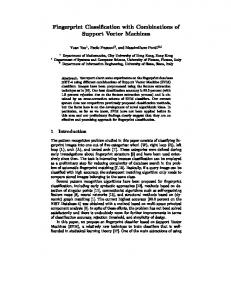
Testability Transformation was first applied to the flag problem [18]. This section considers the particularly difficult variant of the flag problem where the flag variable is assigned within a loop. Several authors have also considered this problem [7, 4]; however, at present, testability transformation offers the most generally applicable solution. Furthermore, this solution is applicable to other techniques such as the chaining method and symbolic execution [10] which are known to be hard in the presence of loop assigned flags. A flag variable is any boolean variable used in a predicate. Where the flag only has relatively few input values (from some set S) that make it adopt one of its two possible values, it will be hard to find a value from S. This problem typically occurs with internal flag variables, where the input state space is reduced, with relatively few ‘special values’ (those in S) being mapped to one of the two possible outcomes and all others (those not in S) being mapped to the other. The fitness function for a predicate that tests a flag yields either maximal fitness (for the ‘special values’) or minimal fitness (for any other value). In the landscape induced by the fitness function, there is no guidance from lower fitness to higher fitness. This is illustrated by the landscape at the right of Figure 2. A similar problem is observed with any k–valued enumeration type, whose fitness landscape is determined by k discrete values. The flag type is the archetype in which k is 2. As k becomes larger the program becomes progressively more testable: provided there is an ordering on the k elements, the landscape becomes
Best case Smooth landscape with ubiquitous guidance toward global optimum.
Acceptable case Rugged landscape with some guidance toward global optimum.
Worst case Dual plateau landscape with no guidance toward global optimum.
Fig. 2. The flag landscape: The needle in a haystack problem. progressively more smooth as k increases. The landscapes in the center and then left of Figure 2 illustrate the effect of increasing k. The problem of flag variables is particularly acute where the flag is assigned a value in a loop and then used later outside the loop. For example, consider the variable flag in the upper left of Figure 3. In this situation, the fitness function computed at the test outside the loop may depend upon values of ‘partial fitness’ computed at each and every iteration of the loop. Many previous approaches to the flag problem breakdown in the presence of loop–assigned flags [4, 7, 19]. These simpler techniques are effective with non-loop-assigned flags. The aim of the loop-assigned flag removal algorithm is to replace the use of a flag variable with an expression that provides better guidance. The algorithm has 2 steps. The first adds two variables: a new induction variable counter is added to the loop to count the number of iterations that take place. The second new variable fitness is a real-valued variable that collects a cumulative fitness score for the assignments which take place during the loop. When applied to code from the upper left of Figure 3, the result of the first step are shown in the upper right of Figure 3. Where “if (flag)” has been replaced with “if (counter == fitness)”. The variable counter measures the number of times the loop passes down the desired path (that which executes the assignment to flag in a way that gives the desired final value for flag). This gives rise to the improved but coarse grained landscape [3] shown in the center of Figure 2. The coarseness comes because loop iteration is deemed either to traverse the desired path (with a consequent increase in accumulated fitness) or to miss this path (with no change in accumulated fitness). A further improvement is possible using an additional transformation that instrument the program to compute, for iterations that fail to traverse the described path, how close the iteration comes to traversing the desired path. The transformed code, shown it the lower section of Figure 3, employs the computation of a “local fitness calculation” (the function local), which captures the proximity of each loop iteration to the desired branch. This produces the smoothest
void f(char a[ELEMCOUNT]) { int i; int flag = 1;
void f(char a[ELEMCOUNT]) { int i; int flag = 1; int counter = 0; double fitness =0.0;
for (i=0; i0) { 17 write(AR[top]); 18 top--; } } 19 else if (cmd==3) { 20 if (top>100) 21 write(1); 22 else write(0); } 23 else if (cmd>=5) 24 f exit=1; } 25 } Fig. 7. A sample C function.
to be executed and R[i] indicates a number of repetitions of this statement. In essence, the transformation has produced a function from the inputs S and R to the value of the fitness function for the problem node. For example, a transformed version of the function from Figure 7 for problem Statement 20 is shown in Figure 9. The transformed function contains the statements that are part of the data dependence subgraph from Figure 8 (statements 4, 13, and 18). The end point is omitted because it does not modify the state. These statements affect the computation of the fitness function associated with problem Statement 20. For statements 13 and 18, for- loops are included because these statements have self-looping data dependences in the data depen-
4
18
13
20 Fig. 8. Data Dependence Subgraph
dence subgraph. After transformation, a search generates different data dependence paths for exploration. A path is represented by S. For each S, the goal is to find values for R such that the fitness function evaluates to the target value. The search uses the existing test generation techniques [15, 31, 43] to find an input on which the fitness function evaluates to the target value in the transformed function. If the target value is achieved, the path is considered a promising path. Otherwise, the path is considered to be unpromising and it is rejected. Finally, promising paths in the transformed program are used to guide the search in the untransformed program. For example, the transformed program for problem Statement 20 from Figure 7, shown in Figure 9, captures the five acyclic paths in the data dependence subgraph of Figure 8. The following table shows these paths and their corresponding inputs path P1 : 4, P2 : 4, P3 : 4, P4 : 4, P5 : 4,
20 18, 13, 13, 18,
20 20 18, 20 13, 20
corresponding input S[1] = 4 S[1] = 4, S[2] = 18 S[1] = 4, S[2] = 13 S[1] = 4, S[2] = 13, S[3] = 18 S[1] = 4, S[2] = 18, S[3] = 13
For each path, the goal is to find values for array R such that the value of the fitness function returned by the transformed function is negative. The search fails for paths P1 and P2 and these paths are rejected. When path P3 is explored, the search finds the values R[1] = 1; R[2] = 101 for which the fitness function evaluates to the negative value in the transformed function. Therefore, path P3 with 101 repetitions of Statement 13 is considered as a promising path. When this
1 float transformed(int S[], int R[]) { int i, j, top; 2 i=1; 3 while (i