Jan 11, 2016 - false positive rate (FPR) reported by M on labeled data. ese values are important, because they give us a feeling of how well M would perform if ...
Jan 11, 2016 - ransomware [14]) and devising more e cient techniques to deliver malicious payloads to victim computers (
tion of a mutant shows its output to have a similar range ... and section VIII presents our conclusions. II. ... Faults exist as incorrect steps .... gave a mutation score of 97.18% on the original set [11][14]. .... as integers in the same way there
how Aspect Oriented Programming (AOP) can be used to modularize service .....
Component software: Beyond Object-oriented programming. Addison-. Wesley ...
Recently genetic programming (GP) has started to show its promise by ... netic
Algorithms + Data Structures = Evolution Programs as the title of his book.
Yuan Yaoi, Paolo Frasconi2, and Massimiliano Pontil3'i. 1 Department of
Mathematics, City University of Hong Kong, Hong Kong. 2 Department of
Systems and ...
Jan 11, 2016 - validate this approach via a large-scale analysis on real-world data. ...... associated with the graphs a
the laboratory setting, opening a separate port for SmartFrog (given the ... if the SmartFrog daemon needs to run as a privileged user such as ârootâ, as is the.
Model Projection, Extended Finite State Machines, Slicing. 1. INTRODUCTION ... The design of models typically occurs earlier in the overall de- velopment ...
Nov 4, 2013 ... Pinocchio Coin: Building Zerocoin from a Succinct. Pairing-based Proof System.
George Danezis. Microsoft Research. Cambridge, UK.
INTRODUCTION TO THE DESIGN AND ANALYSIS OF. ALGORITHMS - Anany
Levitin (Pearson International) Clear and well written and about the right level.
Jul 23, 2010 - Modelling of Spiking Neurons Using GPUs," Application-Specific Systems, ... âR. Stewart and W. Bair, "Spiking neural network simulation: ...
reverse engineering technology of the 1990s. Keywords. Software engineering, reverse engineering, data reverse en- gineering, program understanding ...
Objective: In order to uncover the latent cluster- ing of mobile apps in app stores, we propose a novel tech- nique that measures app similarity based on claimed ...
void f(char a[ELEMCOUNT]) void f(char ...... Rothermel. An empirical study of ... In Raymond T. Ng, Peter A.; Ramamoorthy, C.V.; Seifert, Laurence C.; Yeh, ed-.
transforming into monstrous forms as seen in some movies. On its own ... enabled us to produce humanoid robots with similar levels of articulation as humans.
Loyola University Maryland. Baltimore, MD, USA [email protected]. ABSTRACT. While clone detection and classification research for textual source.
scale e-business solutions that fulfill business goals within a short time-to- .... must collaborate and coordinate its activities with other components in a com-.
Simon Tavaré. 1 University of Sheffield, Sheffield, Great Britain. * [email protected]. There is a large class of stochastic models for which we can simulate ...
Towards Higher Impact Argumentation. Anthony Hunter. â. Dept of Computer Science. University College London. Gower Street, London WC1E 6BT,UK.
distributed system construction well ... Support distributed and heterogeneous
object requests .... Coulouris; Dollimore; Kindberg: Addison Wesley, 2001.
We chose HCI practitioners in the website domain as a sample population to ..... constant comparison method to check the legitimacy of insights created the ...
Technologies for forgetting. Ian Brown ... best way to “forget” personal data is that
it should not be “remembered” in the first place. ... They therefore stop the.
Robert M. Hierons ... [email protected]. Keywords: slicing, transformation, search based software engineering ...... [24] C. Norris and L. L. Pollock.
Chapter 11, in Genetic Programming Theory and Practise, Rick L. Riolo and Bill
... solutions, evolutionary search is effective at finding them (Section 11.6).
Chapter 11, in Genetic Programming Theory and Practise, Rick L. Riolo and Bill Worzel (editors), pp173-188, Kluwer, 2003.
Chapter 11 THE DISTRIBUTION OF REVERSIBLE FUNCTIONS IS NORMAL W. B. Langdon [email protected]
Computer Science, University College, London, Gower Street, London, WC1E 6BT, UK
Abstract
The distribution of reversible programs tends to a limit as their size increases. For problems with a Hamming distance fitness function the limiting distribution is binomial with an exponentially small chance (but non zero) chance of perfect solution. Sufficiently good reversible circuits are more common. Expected RMS error is also calculated. Random unitary matrices may suggest possible extension to quantum computing. Using the genetic programming (GP) benchmark, the six multiplexor, circuits of Toffoli gates are shown to give a fitness landscape amenable to evolutionary search. Minimal CCNOT solutions to the six multiplexer are found but larger circuits are more evolvable.
We shall show the fitness of classical reversible computing programs [Bennett and Landauer, 1985] (where fitness is given by Hamming distance from an ideal answer) is Normally distributed. If the score is normalised so that the maximum score (fitness) is 1 and the minimum n is 0, then the mean is 0.5 and the standard deviation is 1/2 m−1/2 2− 2 . (Where n is the number of input bits and m is the number of output bits.) Almost all genetic programming has used traditional computing instructions, such as add, subtract, multiple, or, and. These instruction 1
sets are not reversible. I.e., in general, it is impossible given a program and its output, to unambiguously reconstruct the program’s input. This is because most of the primitive operations themselves are irreversible. However genetic programming can evolve reversible programs composed of reversible primitives. A number of reversible gates have been proposed [Toffoli, 1980, Fredkin and Toffoli, 1982] which can be connected in a linear sequence to give a reversible gate array, which we will treat as a reversible computer program. At present the driving force behind the interest in reversible computing is the hope that reversible gates can be implemented as quantum gates, leading to quantum coherent circuits and quantum computing. Reversible computing has also been proposed for safety critical applications and for low power consumption or low heat dissipation. In the absence of counter measures, most traditional computer programs degrade information. I.e. knowledge about their inputs is progressively lost as they are executed. This means, most programs produce the same output regardless of their input [Langdon, 2002b]. Suppose a n program has n input bits and m output bits, there are 2m2 possible functions it could implement. However a long program is almost certain to implement one of the 2m constants. That is, the fraction of functions actually implemented is tiny as the programs get longer and worse, the fraction of interesting functions tends to zero. This is due to the inherent irreversibility of traditional computing primitives. In the next section we describe reversible computing in more detail. In reversible computing there is also a distribution of functions which programs tend to as they get longer. Instead of it being dominated by constants, every reversible function is equally likely (cf. Section 11.3). Convergence to this limit is tested in Section 11.5 on the Boolean 6 Multiplexor problem (described in Section 11.4). Section 11.5 shows convergence to the large program limit can be rapid. Despite the low density of solutions, evolutionary search is effective at finding them (Section 11.6). Initial results suggest, CCNOT and traditional computing primitives are similarly amenable to evolutionary search.
2.
Reversible Computing Circuits
A reversible computer can be treated as an array of parallel wires leading from the inputs and constants to the outputs and garbage. In normal operation the garbage outputs are treated as rubbish and discarded by the end of the program. Connected across the wires are reversible gates. Each gate has as many inputs as it has outputs. The gates are reversible, in the sense
3
The Distribution of Reversible Functions is Normal
3 input reversible gate
Inputs
Outputs 5 input reversible gate
constant inputs
Garbage
(scratch memory)
Figure 11.1. Schematic of reversible computer. In normal operation data flows from left to right. However when reversed, garbage and outputs are fed into the circuit from the right to give the original inputs to the program (plus constants).
CCNOT not
swap Inputs
Outputs
A
A xor (B.C)
B
B
C
C
Figure 11.2. Examples of reversible gates. The CCNOT (Toffoli) gate passes all of its inputs directly to its outputs, unless all of the control lines (B and C) are true, in which case it inverts its main data line (A). (The control inputs of a CCNOT gate (B and C) can be connected to the same wire but the controlled wire (A) cannot be directly connected to either control.) CCNOT is complete, in the sense all boolean circuits can be constructed from it.
that it is possible to unambiguously identify their inputs given their outputs (see Figure 11.1). The simplest reversible gate is the identity, i.e. a direct connection from input to output. Also NOT is reversible, since given its output we know what its input must have been. Similarly a gate which swaps its inputs is also reversible (see Figure 11.2). We will mainly be concerned with the controlled-controlled not (CCNOT, Toffoli) gate. Unless all of its control lines are true, the CCNOT gate passes all of its inputs directly to its outputs. However if they are all set, CCNOT inverts the controlled line. CCNOT is complete in the sense, given sufficient CCNOT gates and additional constant inputs and rubbish outputs, a reversible circuit equivalent to any Boolean function from inputs to outputs (excluding constants and rubbish) can be constructed. Since CCNOT can invert 1, the additional inputs can all be 1. Note a single CCNOT gate (plus a constant zero, e.g. provided by us-
4 ing another CCNOT gate to invert a one) can implement the identify function. In C code data[A] = (data[C] & data[B]) ^ data[A]; While it is not necessary for the number of lines set to true, to remain constant across the circuit from left to right, a reversible computer must implement a permutation. To explain what we mean by this, consider the left hand side (of N wires) as an N bit number. There are up to 2N possible left hand patterns. Similarly there are up to 2N possible right hand patterns. The computer provides a mapping from left hand number to right hand number. For the mapping to be reversible, its range and domain must be the same size and a number can only appear once on the right hand side (range), i.e. the mapping must be a permutation. If all N 2N possible numbers are used, only 2N ! of the 2N 2 possible mappings N are reversible. For large N , this means only about 1 in e2 mappings are permutations and hence are reversible. The computation remains reversible up until the garbage bits are discarded. It is at this point that information is lost. It is the deletion of information which means the computation must consume energy and release it as heat. By carefully controlling the deletion of these rubbish bits, it has been suggested that reversible computers will require less energy than irreversible computers. Present day circuits do not approach the lower bound on energy consumption suggested by their irreversibility. I.e. they require much more energy to operate gates, drive connecting wires, etc. than the theoretical bound on energy consumption due to information lost as they run. However in the near term, energy consumption is interesting both for ultra-low power consumption, e.g. solar powered computing, and also because the energy released inside the computing circuit has to be removed as heat. The only way heat is removed at present is by making the centre of the circuit hotter and allowing heat to diffuse down the temperature gradient to the cooler boundaries of the circuit. (Active heat pumps within the circuit have been considered. Electronic refrigerators could be based upon the Peltier electro thermodynamic effect). Even today cooling circuits is a limiting factor on their operation. Increasing circuit clock speeds, despite continued reduction in circuit size, mean heat removal will be an increasing concern. [Bishop, 1997] describes a single channel reversible system for a safety critical control application. By running the system forwards and then backwards and comparing the original inputs with those returned by traversing the system twice, he demonstrated the system was able to detect test errors injected into the system during its operation. (High reliability systems often use comparison between multiple channels to detect errors.)
The Distribution of Reversible Functions is Normal
3.
5
Distribution of Large Reversible Circuits
As with a complete reversible circuit, the action of a single reversible gate across N wires can be treated as a permutation mapping one N bit number to another. Following [Langdon and Poli, 2002],[Langdon, 2002a],[Langdon, 2002b], we can treat the sequence of permutations from the start of the circuit to its end as a sequence of state transitions. The state being the current permutation. We restrict ourselves to just those permutations which can be implemented, i.e. states that can be reached. Each gate changes the current permutation (state) to the next. We can describe the action of a gate by a square matrix of zeros and ones. Each row contains exactly one one. The position of the one indicates the permutation on the output of the gate for each permutation on the input side of the gate. (Note the matrix is row stochastic). Now each gate is reversible. I.e. given a permutation on its output side, there can only be one permutation on its input side. This means each column of the matrix also contains exactly one one. (I.e. the matrix is column as well as row stochastic, i.e. it is double stochastic). We will have multiple ways of connecting our gates or even multiple types of gate, however each matrix will be double stochastic and therefore so too will be the average matrix. Since we only consider implementable permutations, the average matrix is fully connected. If a single gate can implement the identity function, the matrix must have a non zero diagonal element. This suppresses cycling in the limit. If we choose gates at random, the sequence of permutations is also random. Since the next permutation depends only on the current permutation and the gate, the sequence of permutations is a Markov process. The Markov transition matrix is the average of each of the gate matrices, which is fully connected, acyclic and double stochastic. This means as the number of randomly chosen gates increases each of the Markov states becomes equally likely [Feller, 1957]. I.e. in the limit of large circuits each possible permutation is equally likely. When there are many randomly connected gates and the total number of lines N is large, not only is each possible permutation equally likely but (since our reversible gates are complete) all m bit output patterns are possible. Further we will assume that we can treat each output bit as being equally likely to be on as off and almost independent of the others. If fitness f is defined by running the program on every input (i.e. running it 2n times) and summing the number of output bits that match a target (f = Hamming distance) then f follows the n n Binomial distribution 2−m2 Cfm2 . This means most programs have a fitness near the average 12 m2n and the chance of finding a solution is
6 n
2−m2 . While small, this is finite, whereas with irreversible gates (and no write protection of inputs) almost all programs do not solve any non trivial problem [Langdon, 2002b]. We can also use the known uniform distribution to calculate the expected RMS error. Suppose T of the 2n possible fitness cases are run, expected average squared error is q Pthe T 1 Pk 1 RMS = k i=1 T t=1 |Pi (inputt + 2N − 2n ) mod 2m − At )|2 . Where k is the total number of permutations, inputt is the input for the tth test, At = required answer and Pi (x) is the ith permutation of x. As 2m k we can approximate the average behaviour of Pi (t + 2N − 2n ) mod 2m over k cases by i overq2m cases. So the expected average squared error P2m −1 1 PT 2 is RMS = 21m i=0 t=1 |i − At | . If only a few tests with small T values are run (i.e. T 2m and At 2m ) then the expected root mean squared error is bounded by
RMS ≈ 2
VARRMS + RMS
=
VARRMS ≈ SD ≈
v
1 2m
m −1 u 2X u
1 2m
m −1 2X
i=0
i=0
t1
T
T X
1 i2 ≈ 2m 2 t=1 m
T −1 1X 1 2X 1 |i − At |2 ≈ m i2 ≈ (2m )2 T t=1 2 i=0 3
1 m 2 1 m 2 (2 ) − (2 ) 3 4 1 m √ 2 = 0.2886751 2m 2 3
On the other hand if exhaustive testing is carried out and the target values are uniformly spread in the range 0 . . . 2m −1 then RMS ≈ 127√3 2m and SD ≈ 0.23 2m .
4.
6 Multiplexor
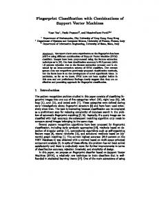
The six multiplexor problem has often been used as a benchmark problem. Briefly the problem is to find a circuit which has two control lines (giving a total of four possible combinations) which are used to switch the output of the circuit to one of the four input lines, cf. Figure 11.3. The fitness of a circuit is the number (0 . . . 64) of times the actual output matches the output given by the truth table. Note fitness is given by number of bits in common between the actual truth table implemented by a program and a given truth table (Hamming distance).
The Distribution of Reversible Functions is Normal
7
D0 D1
Output
D2 D3
A0 A1
4 way switch
Figure 11.3. Six way multiplexor. Only one of four data lines (D0, D1, D2 and D3) is enabled. Which one is determined by the two control lines (A0 and A1).
5.
Density of 6 Multiplexor Solutions
We measured1 the distribution of fitness of randomly chosen CCNOT programs with 0, 1 and 6 additional wires at a variety of lengths, cf. Figures 11.4–11.10. These experiments confirm that there is a limiting fitness distribution and it is Binomial. Further, cf. Figure 11.9, the difference between the actual distribution and the limiting distribution falls rapidly with program length. Also we do not need many spare wires (one is sufficient) to be close to the theoretical wide circuit limit. Only without any spare lines does the limit differ from theory. There are no CCNOT solutions to the six multiplexor problem with less than five gates. One of the smallest solution is shown in Figure 11.11. Notice this does not use any additional wires. While the multiplexor can be solved by CCNOT without additional storage, with six lines only even fitness scores are possible. This also means, even in the limit of long programs, there is a bias towards higher fitness, increasing the mean fitness from 32 to 32.5, cf. Figures 11.4, 11.5, 11.8 and 11.10. It is clear that CCNOT has a nice bias for solving the six multiplexor problem. On average small circuits have above average fitness and in particular (at least with six lines) the chance of solving the problem is far higher for small programs than in the limit of large programs.
6.
Hill Climbing and Evolutionary Solution of the Six Multiplexor Problem
Section 11.3 tells us how many solutions there are but not how easy they are to find. To investigate this we carried out hill climbing and
Figure 11.4. Proportion of circuits composed of controlled-controlled-NOT (CCNOT, Toffoli) gates of each fitness on the 6 multiplexor problem. Solutions have fitness of 64. (At least 100 million random circuits tested for each length.) Since the only wires are those carrying the inputs (i.e. no additional memory) odd fitness values cannot be generated. To simplify the graph these are excluded. 1 0.01 0.0001 1e-06 10 CCNOT solutions 6 10-8
Figure 11.5. Data as Figure 11.4. In Figure 11.4 the large circuit limit is approximated by a Normal distribution with mean 32.5. Here the Binomial distribution approximates the tails near fitness 0 and 64.
9
The Distribution of Reversible Functions is Normal Measurement Long program limit Fraction
0.1 0.01 0.001 0.0001 1e-05 1e-06 0 20 30 40
48
50 100 Number of CCNOT gates
200 0
8
16
56
64
40 32 24 Fitness on 6 Multiplexor
Figure 11.6. Convergence of 6 multiplexor fitness distribution as number of CCNOT gates is increased from 20 towards the large circuit limit (ringed parabola right hand end). (At least million random circuits tested for each length.) One additional memory (garbage) line ensures all output patterns can be implemented and in the large circuit limit are equally likely. I.e. the density of solutions is 2−64 .
population based search on the minimal circuit and a larger circuit. Our results are summarised in Table 11.1. Firstly we compare random search with these two more sophisticated search techniques. Figure 11.10 shows the chance of solving the six multiplexor by random search of CCNOT circuits. From the first solutions composed of 5 gates and no spare lines, the chance rises from about 3 10−8 to a peak of about 10 10−8 at 10 gates, and then falls towards the theoretical (non zero) limit of 5.4 10−20 as the circuit size increases. (No solutions were found in more than 10,000,000 trials with either one or six spare lines.) A local hill climber was run ten times. It mutated exactly one CCNOT gate of the five in the six wire circuit and retained the mutant only if its fitness was better. In seven runs a fitness level of 56 was reached. In two
Table 11.1.
Number of runs solving the six multiplexor problem Configuration Hill climber Population 6 lines 5 CCNOT 0/10 4/10 12 lines 20 CCNOT 1/10 10/10
10
binomial large limit 20 CCNOT 100 CCNOT 2000 CCNOT
Figure 11.7. Distribution of fitness on the 6 multiplexor problem of circuits of CCNOT gates and with 12 lines.
Mean and SD of fitness distribution
40
6 wires 7 wires 12 wires
38
36
34 6 wire Mean limit 32.5 32
30.
Mean limit 32.0
1
2
3 4 5 6 7 8 101215 20 30 4050 100 Number of CCNOT
200
500
1000
2000
Figure 11.8. The fitness distribution of small CCNOT circuits are asymmetric with mean near 40. As number of Toffoli gates is increased, both mean and standard deviation converge to theoretical binomial limits (32 and 4), except for circuits without spare wires, in which case the mean converges to 32.5.
11
The Distribution of Reversible Functions is Normal
Total variation distance
1
6 wires 7 wires 12 wires
0.1
0.01
Noise
0.001
0
50
100 Number of CCNOT gates
150
200
Figure 11.9. Discrepancy between measured distribution of fitness on CCNOT 6 multiplexor problem and large circuit limit (calculated as total variation distance [Rosenthal, 1995]). Rapid convergence to theoretical limit as program size increases is shown. We would expect more spare lines to mean bigger programs are needed for convergence. The plots are reminiscent of exponential decay shown for non reversible programs [Langdon, 2002a] suggesting group theory might lead to results on the rate of convergence.
of the seven runs the hill climber reached fitness 56 significantly2 faster than random search could be expected to. In seven of the remaining runs there is no significant difference between the hill climber and random search. (However random search always has a chance of solving the problem. While the hill climber was stuck at local optima and could never proceed.) In the remaining run, the hill climber took significantly longer to reach fitness level 48. Our hill climber found one solution in ten runs, when the number of CCNOT gates was increased to 20 and six spare lines were added. Six of the runs attained a score of 56, two runs 48 and the last 52. None of these nine runs first reached its final fitness level significantly faster or slower than random search might be expected to. Except again random search might improve, whereas the hill climber was stuck at local optima and could never proceed. (Each 20 CCNOT 12 wire program has 20×(2×(12−2)+(12−3)) = 580 or 20×3×(12−2) = 600 neighbours, so our hill climber will take on average no more than 4185 attempts to try
12 1e-07
6 lines, fitness=64
9e-08 8e-08 7e-08
Fraction
6e-08 5e-08 4e-08 3e-08 2e-08 1e-08 0
1
2
3 4 5 6 7 8 101215 20 30 4050 100 Number of CCNOT
200
500
1000
2000
Figure 11.10. Measured density of solutions on CCNOT 6 multiplexor problem. (Based on measurements of at least 100,000,000 random circuits of each length. In one million random samples at each length, with either one or six spare lines no solutions were found.)
them all, cf. The Coupon Collector’s problem [Feller, 1957, page 284]. All runs had many more trials than this.) In contrast the search space turns out to be very friendly to evolutionary search. Using the same mutation operator and a population of 500 (see also Table 11.2) in four out of ten runs minimal solutions to the six multiplexor were found. (I.e. five CCNOT without spare wires). These solutions took between 20 and 100 generations. In the remaining six runs fitness level 56 was reached (in five cases significantly faster than random search). Introducing six spare wires and extending the circuits from five to 20 CCNOT makes the problem significantly easier. Ten out of ten runs (with the same population size etc.) found solutions. The solutions were found after 30–220 generations. This is significantly better than hill climbing and population search of the smaller circuit size. The effort [Koza, 1992, page 194] required to find a non-minimal reversible solution to the six multiplexor using a population approach (87,000) is somewhat similar to that required by genetic programming to find a non-reversible one [Koza, 1992, Table 25.2]. In other words, using CCNOT with spare lines has not been shown to be uncompetitive with existing approaches.
13
The Distribution of Reversible Functions is Normal Table 11.2.
Parameters for Multiplexor Problem
Objective: Inputs: Functions set: Fitness cases: Fitness: Selection: Pop size: Program size: Parameters:
Termination:
Find a reversible function whose output is the same as the Boolean 6 multiplexor function D0 D1 D2 D3 A0 A1 (plus either 0 or 6 “true” constants) CCNOT All the 26 combinations of the 6 Boolean arguments number of correct answers Tournament group size of 7, non elitist, generational 500 5 or 20 CCNOT (Toffoli) reversible gates 100% mutation (Exactly one CCNOT gate is randomly chosen. One of its three wires is chosen at random, and replaced by a randomly chosen, different, but legal, wire.) fitness=64 or maximum number of generations G = 500
D0 D1 D2 D3 A0 A1
CC CC CC CC CC 0
3
2
2
0
1
2
4
5
2
4
4
3
0
5
Figure 11.11. Example evolved minimal circuit (left) of controlled-controlled-NOT (CCNOT, Toffoli) gates implementing a six way multiplexor. Genetic representation on right. Two address lines direct one of the four data inputs to the output. Circles with crosses indicate controlled wire. Note there are no additional memory (garbage) lines and only five gates are required.
7.
Discussion
It is important to realise the limiting distribution results hold in general for reversible computing. Not just for the six multiplexor or similar problems and for any reversible gate, not just the Toffoli (CCNOT) gate. An interesting extension would be quantum computing. Random matrices theory may give a formal bound on the size of circuits needed to approach the limiting distribution. The benchmark can be solved with no spare wires. Indeed [Toffoli, 1980, page 636] describes a set of gates for which no more than m spare wires are needed for any finite reversible function. However allowing modest increases in the size of solution by allowing more gates and spare wires appears to make the fitness landscape more evolvable. I.e. easier for evolutionary search to find solutions. It is not clear whether addi-
14 tional gates or wires or both is primarily responsible. In our example at least, and we suggest perhaps to other problems, insisting upon minimal solutions rather than sufficient solutions, which may be bigger, makes the problem unnecessarily hard. While NFL [Wolpert and Macready, 1997] applies to reversible computing, we expect evolutionary search also to be better than hill climbing and random search when used with other reversible gates, such as the Fredkin gate, on this and similar problems. The number of programs or circuits of a given size increases exponentially with circuit size. Thus average behaviour across all programs is dominated by the behaviour of the longest programs. Almost all of these will behave as the limiting distribution suggest. Thus considering only the limiting distribution is sufficient to describe the vast majority of programs. Where spare wires are included, for most programs, the Binomial distribution can be approximated by a Normal distribution with the same mean and variance. I.e. where fitness is given by a Hamming distance, the average fitness is 12 m2n and the variance is 1/2 1/2 m2n . If we normalise fitness to the range 0 . . . 1, then the mean becomes 0.5 −n 2 and the standard deviation is 22√m . Even with modest numbers of input and output wires, the Hamming fitness distribution becomes a needle, with almost all programs having near average fitness. In non-trivial problems n and m rapidly become too large to allow exhaustive testing. However the limiting distribution still applies. In the limit the chance of a random program passing non-exhaustive testing is given by the number of bits which are checked. I.e. if T tests are run and only a p precision answer is needed, the chance of passing a test case is 2−p . The chance of passing all the test cases is 2−T ×p . But note that, randomly passing the test cases gives no confidence that the program will generalise. If an additional independent test is added, the chance of randomly passing it is only 2−p [Langdon and Poli, 2002]. In contrast general solutions have been evolved via limited numbers of test cases by genetic programming [Langdon, 1998] suggesting GP has a useful bias for problems of interest.
8.
Conclusions
As with traditional computing, as reversible circuits get bigger the distribution of their functionality converges to a limit. Therefore their fitness distribution must also tend to a limit. Table 11.3 summarises the limit (with many wires) for fitness functions based on Hamming distance and root mean error squared. In the limit, every implementable
15
The Distribution of Reversible Functions is Normal Table 11.3.
Distribution of Fitness of Large and Wide Reversible Circuits
permutation is equally likely. Note, unlike traditional computing, in the limit there is a finite chance of finding a solution. Experiments on the six multiplexor problem have found solutions, including minimal solutions, cf. Figure 11.11. These experiments suggest the fitness landscape is amenable to evolutionary search, particularly if non-minimal solutions are allowed. Which in turn suggests the use of variable length evolution. Performance with CCNOT (Toffoli) gates is similar to that of genetic programming with non reversible programs. Simple hill climbing is liable to become trapped at sub optima, particularly if constrained to search for minimal solutions. We suggest that the common emphasis on minimal solutions is misplaced. These examples provide additional evidence that requiring tiny solutions hurts evolvability (and other search techniques). There may only be one smallest program but there are exponentially many larger solutions.
Acknowledgments I would like to thank Tom Westerdale, Ralph Hartley, Tina Yu, Wolfgang Banzhaf, Joseph A. Driscoll, Jason Daida, Lee Spector and Tracy Williams.
Notes 1. In all the six multiplexor experiments we used speed up techniques based on those described in [Poli and Langdon, 1999]. 2. All significance tests in Section 11.6 use a 5% two tailed test.
References [Bennett and Landauer, 1985] Bennett, Charles H. and Landauer, Rolf (1985). Fundamental physical limits of computation. Scientific American, 253(July):48–56.
16 [Bishop, 1997] Bishop, Peter G. (1997). Using reversible computing to achieve fail-safety. In Proceedings of the Eighth International Symposium On Software Reliability Engineering, pages 182–191, Albuquerque, NM, USA. IEEE. [Feller, 1957] Feller, William (1957). An Introduction to Probability Theory and Its Applications, volume 1. John Wiley and Sons, New York, 2 edition. [Fredkin and Toffoli, 1982] Fredkin, Edward and Toffoli, Tommaso (1982). Conservative logic. International Journal of Theoretical Physics, 21(3/4):219–253. [Koza, 1992] Koza, John R. (1992). Genetic Programming: On the Programming of Computers by Means of Natural Selection. MIT Press. [Langdon, 2002a] Langdon, W. B. (2002a). Convergence rates for the distribution of program outputs. In Langdon, W. B., et. al., editors, GECCO 2002: Proceedings of the Genetic and Evolutionary Computation Conference, pages 812–819, New York. Morgan Kaufmann Publishers. [Langdon, 2002b] Langdon, W. B. (2002b). How many good programs are there? How long are they? In Rowe, Jonathan, et. al., editors, Foundations of Genetic Algorithms VII, Torremolinos, Spain. Morgan Kaufmann. [Langdon and Poli, 2002] Langdon, W. B. and Poli, Riccardo (2002). Foundations of Genetic Programming. Springer-Verlag. [Langdon, 1998] Langdon, William B. (1998). Genetic Programming and Data Structures. Kluwer. [Poli and Langdon, 1999] Poli, Riccardo and Langdon, William B. (1999). Sub-machine-code genetic programming. In Spector, Lee, et. al., editors, Advances in Genetic Programming 3, chapter 13, pages 301–323. MIT Press. [Rosenthal, 1995] Rosenthal, Jeffrey S. (1995). Convergence rates for Markov chains. SIAM Review, 37(3):387–405. [Toffoli, 1980] Toffoli, Tommaso (1980). Reversible computing. In de Bakker, J. W. and van Leeuwen, Jan, editors, Automata, Languages and Programming, 7th Colloquium, volume 85 of Lecture Notes in Computer Science, pages 632–644, Noordweijkerhout, The Netherland. Springer-Verlag. [Wolpert and Macready, 1997] Wolpert, David H. and Macready, William G. (1997). No free lunch theorems for optimization. IEEE Transactions on Evolutionary Computation, 1(1):67–82.