Modeling and validation of a new generic virtual ...

Modeling and validation of a new generic virtual optical sensor for ADAS prototyping D. Gruyer, M. Grapinet, P. De Souza

Abstract— In the early design stages of embedded applications, it becomes necessary to have a very realistic simulation environment dedicated to the prototyping and to the evaluation of these Advanced Driving Assistance Systems (ADAS). This Numerical simulation stage is gradually becoming a strong advantage in active safety. The use of realistic numerical models enabling to substitute real data by simulated data is primordial. For such virtual platform it is mandatory to provide physics-driven road environments, virtual embedded sensors, and physics-based vehicle models. In this publication, a generic solution for cameras modelling is presented. The use of this optical sensor simulation can easily and efficiently replace real camera test campaigns. This optical sensor is very important due to the great number of applications and algorithms based on it. The presented model involves a filter mechanism in order to reproduce, in the most realistic way, the behaviour of optical sensors. The main filters used in ADAS developments will be presented. Moreover, an optical analysis of these virtual sensors has been achieved allowing the confrontation between real and simulated results. An optical platform has been developed to characterize and validate any camera, permitting to measure their performances. By comparing real and simulated sensors with this platform, this paper demonstrates this virtual platform (Pro-SiVIC™) accurately reproduces real optical sensors’ behaviour.

I. INTRODUCTION For some decades, different researches have been done to improve the safety of road environments and reduce the risk of unsafe traffic areas. Initially they mainly focused both on the perception surrounding a vehicle (local perception with embedded sensors) and its potential reaction on hazardous situation. To provide a complete string of functionalities, it becomes necessary to make a prototype and an implementation of optical sensors embedded in vehicles or infrastructures. Unfortunately, this implementation of invehicle sensors is often very constraining. Indeed, the prototyping and the test of many perception algorithms request heavy hardware and software supports. To achieve Manuscript received january 31, 2012. This work was supported and funded by FUI eMotive French project. Dominique Gruyer, LIVIC (IFSTTAR), 14 route de la minière, bat. 824, 78000 Versailles-Satory, France (phone: (+33) 1 40 43 29 07; fax: (+33) 1 40 43 29 31; e-mail: [email protected]). Mélanie Grapinet, LEMCO (IFSTTAR), 25 allée des Marronniers, 78000 Versailles-Satory, France (phone: (+33) 1 30 843951; e-mail: [email protected]). Philippe Desouza, CIVITEC ; 8rue Germain Soufflot, 78180Saint Quentin en Yvelines, France (e-mail: [email protected]).

such perception system, additional developments and implementation of numerous expensive embedded devices are required. Therefore, in early design stages, it becomes necessary to have a very realistic simulation environment dedicated to the prototyping and to the evaluation of these Advanced Driving Assistance Systems (ADAS). This numerical simulation stage is gradually becoming a strong advantage in active safety [1][2][3][4]. The realistic numerical models enabling to substitute real truth by simulated truth is primordial. For such virtual platform it is mandatory to provide physics-driven road environments, virtual embedded sensors, and physics-based vehicle models [5]. To achieve a physically realistic simulation of an optical camera, lighting computation is a key challenge, since a biased input to the camera will unavoidably lead to erroneous camera output. Ray Tracing [6], Radiosity [7] and Monte Carlo Analysis [8] algorithms are identified approaches that focus on different goals. To model the full optical chain, these methods are often combined together with adaptations or improvements yet are too computationally heavy. Our objective is to provide to the user a generic optical modelling that is well suited to real time ADAS prototyping. In this publication, the chosen solution for generic optical sensor is presented, including the rendering stage. Then the validation of the optical model is presented using a characterization platform. By comparing real and simulated sensors with this platform, this paper demonstrates that ProSiVICTM platform accurately reproduces real optical sensors’ behaviour. II. ARCHITECTURE FOR REALISTIC CAMERA MODELLING A. Introduction In order to compute a physical-driven camera simulation, realistic information must be applied to the camera model. It must be kept in mind that the optical information to be provided to a camera may be different to human vision. Thus, the rendering stage should compute realistic spectral luminance data based on the geometrical description of the scene, lighting conditions, and material properties. Luminance is evaluated at the centre of the camera’s entrance pupil, then, the stages of the camera modelling simulate how the different stages of a real camera would

operate. Image signal is as generic as possible, to allow both a large range of applications and maximum of flexibility.

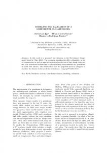
Fig. 1: General view of the camera modelling under SIVIC

B. Sensors simulation engine To model a broad range of optical sensors with different levels of accuracy, a mechanism of adapted rendering has been implemented in a simulation engine, called multirendering. It then becomes possible to define and use different rendering plug-ins adapted to specific requirements. For instance a basic graphical rendering for an optical sensor, or a more realistic optical sensor with HDR (High Dynamic Range) textures, shadows, filters and tone mapping. Currently, three optical rendering techniques are available. The first one provides a classical 3D graphical engine rendering, the second one provides a better shadow and light management, and the last one developed in the framework of the eMotive project improves the physical realism of light interaction with objects. The engine allows applying various post-processing effects to complete the rendering. C. Mechanisms for efficient environment modelling 1) Lighting and interaction with object Beyond the realistic shadowing – that allows increasing scene dynamic and improving contrast realism – an important part of the rendering relies on the lighting computation itself, specifically when addressing complex situations like sunset/sunrise or night driving.

Fig. 2: multi-rendering and filters mechanism (a: initial image, b: noise, c: noise and depth of field, d: noise, DoF and fog)

Addressing this issue implies to consider at the same time the properties of the light sources (especially their intensity angular diagram), and the reflective properties of surfaces. Realistic rendering of surfaces has been abundantly addressed in the past years and perhaps decades, with very different focuses. The objective of Pro-SiVIC™ being to offer an interactive simulation, the two main criteria for developing this rendering stage were computation efficiency, and ease to modify material properties. Contrary to classical driving simulator, the objective is to simulate correct image dynamic rather that create details that make simulation acceptable by human eye. BRDF (Bidirectional Reflectance Distribution Function) descriptions are now commonly used to describe the behaviour of homogeneous reflective surfaces, and various works have been carried out to compare the accuracy of parametric BRDF models for several measured surfaces such as in [9]. In automotive application, the classes of materials involve plastic, metal (sometimes painted), and rougher surfaces such as road concrete or back-scattering materials such as sign-boards and road paint. To cover these classes of materials, Lafortune model [10], Cook-Torrance [11] and the classical Blinn-Phong [12] have been implemented using shader programs. For most materials, the modelled BRDF does not have to be accurate for every incident angle : for example, road surface will most of the time be viewed between 90° and 20°, and sign boards are mostly lighted around back-scattering angles for night driving. Therefore, this reduces the need for more complex BRDF representations. In order to improve and to complete the sensor simulation engine, some plug-ins (filters) have been developed. Two types of filters are provided. The first one is dedicated to the improvement of the environment quality rendering. The second one is focused on the camera modelling (see fig 2). About the first set of filters, the most important are dedicated to the simulation of the weather conditions. Among these climate filters, the fog and the rain filters (waterfall and raindrops) are the most useful. 1) Filters for the rain The rain is modelled by two filters. The first filter reproduces the waterfall and the second simulates the drops of water on a camera lens or a glass (figure 3). The object with the type mgRainActor simulates rainfall or snow in the rendered images. It performs the simulation and rendering of each raindrop trajectories (figure 3b). For the second type of filter, the rain drops are computed in real time with the use of a post processing filter. This filter computes a new texture from the initial camera rendering. For each drop, the original image is inverted in order to simulate the real effect of a rain drop. Moreover, this dynamic texture is computed for a configurable size, a min drop size, a max drop size and fades parameters (speed at which the drops flow and disappear). (figure 3a).

omnidirectional camera model. Each model is tuned with the matrix size, the focal length, and a set of filters. 1) Generic camera a) Fig. 3. a) Drops rain simulation, b) Rain with particles and wet road with environment reflection.

2) Filters for the fog The fog can be tuned according to 3 different setups. The first one is a homogeneous fog computed with the Koschmieder law [19]. The second one uses a post processing technique in order to compute a non homogeneous fog with the merging of the Koschmieder law and the Perlin noise (figure 4b). Unfortunately, at this moment, this second model of fog can only be used for static camera (static point of view). The last one already uses the Koschmieder law but only in a closed area. This last fog modelling is very interesting because it is possible to move it during the simulation (figure 4a).

Filters for blur and glow effects

One can often observe in the images recorded with real cameras the appearance of burs around areas of high light energy. This glare is related to the optic and the contribution of video sensor technology (CMOS or CCD). To simulate such artefacts, Pro-SiVICTM platform offers a post processing plug-in called mgGlowFilter. The object with the type mgGlowFilter manages simulation of gain control and sensor blooming, based on image histogram balance (figure 7a). To complete this function and benefit from HDR textures (High Dynamic Range) representing scene real luminance, a tone mapping filter simulates the sensitivity curve of the sensor. The scene’s dynamic range is in this manner degraded to sensor’s dynamic range.

Fig. 6. HDR rendering with an original factor of 0.4 and 1.0 Fig. 4. a) Homogeneous fog in a specific area, b) Homogeneous and static non homogeneous fog modelling [6]

3) Filter for the night lights To complete the filter with type "weather", functionalities are available with the light sources management. These functionalities allow simulating the lighting during night period. In order to use this type of lighting (lamps, headlights), a light mask mechanism is available. This mechanism is not achieved by pixel but by using an effective 3D area of illumination. The light rendering is tuned with an attenuation coefficient and a field of lighting angle. In addition, the light mask is used to modulate the light output. (Figure 5)

The use of this information is very important because it allows computing luminance in real units, thus simulating physical effects that would not appear in a simple RGB colour simulation. a)

Filter for the noises

At this moment, three type of noise are available: Pulse Noise : The following transform is applied to the brightness of the pixels:  x + p1 si u ≤ p 2  f ( x ) =  x si p 2 < u < 1 − p 2  x − p si u ≥ p 1 2 

where u is drawn for each pixel according to an uniform distribution on[0 ; 1] Additive Gaussian noise: f ( x) = x + p1 .n , where n is drawn according to a standard normal distribution. Fig. 5. a) SiVIC’s car lights in night condition, b) Pro-SiVIC™ camera output, using several light sources and reflective materials.

D. Camera modelling Once the rendering of the environment is done, it is necessary to take into account the imperfections and the working limits of the optical sensor. Currently, there are two camera models available: a generic camera model, and an

Multiplied uniform noise: f ( x) = (1 + p1 ⋅ (u − 0,5)) ⋅ x , where u is drawn according to an uniform law on [0 ; 1] interval. b)

Filter for the colour management

The sivicFiltreCouleurs plug-in applies a homogeneous transformation matrix on the colours of the rendered image. This allows obtaining a lot of efficient effects: scale and

offset brightness and saturation, hue rotation, change of colour space (RGB NTSC, PAL RGB, YUV, YIQ, YCbCr, CMY). An affine transformation is applied to the RGB vector, using a 4x4 matrix as described in [13]. c)

Filter for lens distortion

The sivicFiltreDistorsion plug-in allows post-processing the image to simulate the distortion due to the camera optic defaults (observed distortion from ideal or a pinhole camera). For each pixel in the output image, the pixel coordinates are translated into distance from the projection point on the sensor surface and converted to polar coordinates. The following nonlinear transformation is then applied to the coordinate r:

(

r ' = r 1 + k1 .r 2 + k 2 .r 4

)

The colour of the input pixel with (r, θ) polar coordinates relative to the projection centre is then assigned to the output. d)

use of six cameras has been chosen. From the rendering stage of these 6 cameras, a new image is generated by processing and merging them (figure 8a)). This technique is interesting because it can compute a 360° image and it is possible to provide an accurate depth map in order to quantify the quality of image processing algorithm. Unfortunately, the time consumption is pretty high – realtime is less likely to be obtained. A second approach has been developed in order to provide a generic framework for the modelling of the omnidirectional camera.

Fig. 8. a) Rendering of a fisheye camera, b) Rendering of an omnidirectional camera

Filter for the depth of field

The SiVIC platform offers two ways in order to add postprocess effect to simulate the “Depth Of Field” in the initial rendered image. These techniques are developed in two post-processing plug-ins. sivicFiltreDOF enables a physically realistic simulation of the Depth Of Field phenomenon based on the dimensions and properties of the “real” optical device. The confusion circle is evaluated for every point, and a "stain" of appropriate size is created in the image output. This simulation is realistic for the price of a pretty heavy impact on performance. mgDOFFilter allows to feign the phenomenon of Depth Of Field by performing a mixture between the original image and a blurred version of it, dependant on the distance, and living a clear focus range. Though the filter does not fairly reflect a physical phenomenon, it provides a convincing result for the viewer and offers good performance (figure 7).

The principle of this second technique is to duplicate the hardware configuration of a true omnidirectional camera (figure 8b)). To achieve this modelling, it is necessary to use a mesh representing the desired shape (sphere, cone, parabola ...). Once this mesh is completed, the environment will be reflected above. For rendering this distorted reflection on the mesh, we finally use a camera with the lens oriented toward the shape reflecting the environment. The figure 9 shows the modelling of a real omnidirectional sensor. The results obtained with this model have proved the efficiency of this approach.

Fig. 9. Modelling of a real omnidirectional camera III. COMPARISON AND VALIDATION

Fig. 7. a) Camera rendering with glow filter, noise and de saturation, b) Depth of Field filter

1) Omni directional cameras To extend the range of simulated cameras in the SiVIC platform, a first simulation technique has been used in order to provide a fisheye camera. Due to the limit of the image rendering with the OpenGL library, a technique based on the

In order to validate the optical sensor modeling developed in the pro-SiVICTM platform, a set of tests has been made using a real laboratory for characterization of optical sensors. This real platform is described in [14]. The validation stage is mainly focused on focal length, distortion [15], vignetting [16] and sensor linearity [17]. Thus, two types of test targets have been used: Dot charts and Retro-lighting chart. Figure 10 shows the pictures of the test targets given by three real and simulated optical systems. In the order, downward, are illustrated the pictures obtained from SPC1030NC webcam, CM040MCL sensor and GE040CB sensor. For each of these three sensors, real system output is

located to the left and simulated system output is located to the right. Table 2: Distortion coefficients k1 and k2

Distortion measurement is obtained with the following considerations. The position of a dot center in the observed image is also known in the undistorted image. For any other point, the undistorted position can be interpolated with a high degree polynomial.

Fig. 10. Pictures of the dot and retro-lighting charts for the real system (on the left) and simulated system (on the right).

These cameras have been modeled in Pro-SiVIC™ using real calibration information, and the simulated images of these charts have been recorded. Then, for each system, the correspondence between the real and simulated system has been analyzed. In the following figures, the results obtained are presented according to the position on the half-diagonal (center - corner) of the test target, named thus radial field position. The blue curves present the real system while the red dashed curve refers to the simulated system resulting from the Pro-SiVIC™ software. The relative error is represented by the green curve. A. Focal length The picture of each system is analyzed and allows obtaining the real values of the focal length. Considering the uncertainties, a good concordance between the values provided by the manufacturer and the measured ones is observed. The same analysis is done on the pictures obtained from the simulated sensors. The table 1 shows the results for the real and simulated optical systems. The analysis of focal length shows excellent matching between the real and simulated systems.

Table 1: Focal length for real and simulated systems with their uncertainty (all values are expressed in mm)

B. Distortion First, the two distortion coefficients k1 and k2 of the distortion equation are determined from measurements of a “checkered pattern” using a real camera. These coefficients are then used to define the parameters to be used in the ProSiVIC™ camera model, and the measurement of distortion curves is performed on simulated and real systems. The results of distortion measurements are summarized on figure 11.

Fig. 11. Measured distortion with (a) Philips SPC1030NC webcam; (b) JAI CM040MCL Camera; (c) JAI GE040CB Camera.

The ratio between the distance of a point to the image center in the observed image and the theoretical image is a relative measure of distortion. In the figure 11, three graphics (a; b; c) illustrate the ratio between the ideal and distorted position for the real and simulated systems. Three graphics (d; e; f) represent the error calculated between the two optical systems for each sensor. The relative error can be described as follows: • For radial field position values smaller than 60%, the relative error is very low. • For radial field position values higher than 60%, a little difference appears but remains small. The error increases with radial field position, which could have been expected regarding the limited number of polynomial coefficients used for fitting. At the edge of the field, an error below 1% appears between the two systems. This error is likely to be an acceptable result. C. Vignetting In the figure 12, we present the fall-off profile of the illumination on three graphics (figure 12a,b,c). Three graphics (figure 12d,e,f) represent the error calculated between the real and virtual optical systems for each sensor. Moreover, the relative error shows an excellent simulation of the vignetting. In the corners, a small error appears in the model. This error is smaller than 1%.

systems, real tests could be only performed for the final validation step. This challenge has shown that Pro-SiVIC™ appears as a valuable solution for the development of active safety systems. At the sight of these results, it is expected ProSiVIC™ will allow automotive majors and suppliers to provide to their customers more reliable and safer products. REFERENCES

Fig. 12. Measured vignetting with (a) Philips SPC1030NC webcam; (b) JAI CM040MCL Camera; (c) JAI GE040CB Camera.

D. Sensor linearity The tone curve is a non-linearity function that characterizes the grey level in function of the exposure. In this case, the retro-lighting chart is used, thus the sensor is characterized with fifteen exposures. The following curves (figure 13) of the tone curve are obtained by a webcam Philips SPC1030NC and a sensor CM040MCL. In this study only the camera behaviour has been addressed. The quality of the rendering is another issue depending of the graphical modelling of the environment. A first study has been made in [18] concerning this topic for road marking detection.

[1]

[2]

[3]

[4]

[5]

[6] [7] Fig. 13. Measured tone curve with (a) Philips SPC1030NC webcam; (b) JAI CM040MCL Camera.

[8]

IV. CONCLUSION AND FUTURE WORKS

[9]

In its current state of development, SiVIC is operational and offers a large set of functionalities making it possible to model and test various advanced sensors. It can reproduce, in the most faithful way, the reality of a situation, the behaviour of a vehicle and the behaviour of the sensors which can be embedded inside the vehicle. The camera models provided in the SiVIC platform has shown their efficiency in a lot of projects for the prototyping of algorithms based on images processing. These applications include the obstacle detection, the road markings detection and tracking, the image restoration in degraded condition. The three optical systems were characterized and simulated in the software Pro-SiVIC™. This paper demonstrates that the numerical simulations performed with the software Pro-SiVIC™ accurately reproduce real tests performed with real optical sensors. These very encouraging results allow relying with much more confidence on ProSiVIC™ simulation, and a large part of the real tests may subsequently be avoided and replaced by numerical simulations. Hence for the development of the active safety

[10]

[11] [12]

[13]

[14]

[15] [16] [17]

M. Nentwig, M. Stamminger, “Hardware-in-the-loop testing of computer vision based driver assistance systems”, Intelligent Vehicles Symposium (IV 2011), Baden-Baden, 5-9 June 2011, Germany. D. Gruyer, S. Glaser, R. Gallen, S. Pechberti, N. Hautiere, “Distributed Simulation Architecture for the Design of Cooperative ADAS”, accepted in FAST-ZERO (Future Active Safety Technology) 2011, Tokyo, Japan, September 5-9, 2011. D. Gruyer, S. Glaser, B. Vanholme, B. Monnier, « Simulation of vehicle automatic speed control by transponder-equipped infrastructure », IEEE ITST 2009, 20-22 October 2009, Lille, France. D. Gruyer, S. Glaser, B. Monnier, “SiVIC, a virtual platform for ADAS and PADAS prototyping, test and evaluation”, in the proceedings of FISITA’10, Budapest, Hungary, 30 may-4 june 2010. D. Gruyer, C. Royere, N. du Lac, G. Michel et J-M. Blosseville, "SiVIC and RTMaps®, interconnected platforms for the conception and the evaluation of driving assistance systems", ITSC'06, october 2006, London, UK. Andrew S. Glassner, “An introduction to ray tracing” Londres : Academic press limited, 1989. M. Cohen and J. Wallace. “Radiosity and Realistic Image Synthesis”. Academic Press Professional, Cambridge, 1993. E. Lafortune, “Mathematical Models and Monte Carlo Algorithms for Physically Based Rendering”. PhD thesis, Katholieke Universiteit Leuven, Belgium, Feb. 1996. A. Ngan, F. Durand, W. Matusik, “Experimental Analysis of BRDF Models”, Eurographics Symposium on Rendering (EGSR2005), 29 june – 1st july, Konstanz, Germany, 2005. E. Lafortune, S-C. Foo, K.E Torrance, D. Greenberg, “Non-linear approximation of reflectance functions”, Siggraph97, 5-7 august, Los Angeles, USA, 1997. L. R Cook., K. E. Torrance, “A reflectance model for computer graphics”, ACM Transactions on Graphics (TOG), 1982. James F. Blinn. "Models of light reflection for computer synthesized pictures". Proc. 4th annual conference on computer graphics and interactive techniques, New-York, USA, 1977. D. Gruyer, N. Hiblot, P. Desouza, H. Sauer, B. Monnier, “A new generic virtual platform for cameras modeling”, in proceeding of International Conference VISION 2010, 6-7 october 2010, Montigny le Bretonneux, France. M. Grapinet, P. Desouza, J.C. Smal, J.M. Blosseville, “Characterization and simulation of optical sensors”, accepted in TRA 2012 conference, 23-26 April 2012, Athens, Greece. Brown DC , "Decentering distortion of lenses." Photogrammetric Engineering. 7: 444–462, 1966. W.J. Smith, “Modern optical engineering: the design of optical systems”, Fourth Edition, McGraw-Hill Companies, 2008. International Standard ISO14524(2009), Photography -- Electronic still-picture cameras — Methods for measuring opto-electronic conversion functions(OECFs).