Monitoring and Damage Detection in Structural Parts of ... - InTechOpen

0 9 Monitoring and Damage Detection in Structural Parts of Wind Turbines Andreas Friedmann, Dirk Mayer, Michael Koch and Thomas Siebel Fraunhofer Institute for Structural Durability and System Reliability LBF Germany 1. Introduction Structural Health Monitoring (SHM) is known as the process of in-service damage detection for aerospace, civil and mechanical engineering objects and is a key element of strategies for condition based maintenance and damage prognosis. It has been proven as especially well suited for the monitoring of large infrastructure objects like buildings, bridges or wind turbines. Recently, more attention has been drawn to the transfer of SHM methods to practical applications, including issues of system integration. In the field of wind turbines and within this field, especially for turbines erected off-shore, monitoring systems could help to reduce maintenance costs. Off-shore turbines have a limited access, particularly in times of strong winds with high production rates. Therefore, it is desirable to be able to plan maintenance not only on a periodic schedule including visual inspections but depending on the health state of the turbine’s components which are monitored automatically. While the monitoring of rotating parts and power train components of wind turbines (known as Condition Monitoring) is common practice, the methods described in this paper are of use for monitoring the integrity of structural parts. Due to several reasons, such a monitoring is not common practice. Most of the systems proposed in the literature rely only on one damage detection method, which might not be the best choice for all possible damage. Within structural parts, the monitoring tasks cover the detection of cracks, monitoring of fatigue and exceptional loads, and the detection of global damage. For each of these tasks, at least one special monitoring method is available and described within this work: Acousto Ultrasonics, Load Monitoring, and vibration analysis, respectively. Farrar & Doebling (1997) describe four consecutive levels of monitoring proposed by Rytter (1993). Starting with „Level 1: Determination that damage is present in the structure“, the complexity of the monitoring task increases by adding the need for localising the damage (level two) and the „quantification of the severity of the damaged“ for level three. Level four is reached when a „prediction of the remaining service life of the structure“ is possible. By using the monitoring systems described above, in our opinion only level 1 or in special cases level 2 can be attained. For most customers, the expected results do not justify the efforts that have to be made to install such a monitoring system. In general, our work aims at developing a monitoring system that is able to perform monitoring up to level 4. Therefore, we think it is necessary to combine different methods. Even though the different monitoring approaches described in this paper differ in the type

www.intechopen.com

208 2

Fundamental and Advanced Topics Will-be-set-by-IN-TECH in Wind Power

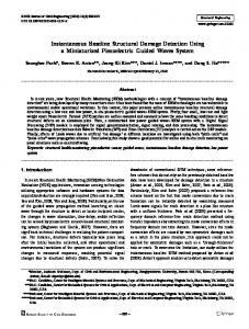
of sensors used or whether they are active or passive, local or global methods, their common feature is that they can be implemented on smart sensor networks. The development of miniaturized signal processing platforms offer interesting possibilities of realizing a monitoring system which includes a high number of sensors widely distributed over the large mechanical structure. This approach should considerably reduce the efforts of cabling, even when using wire-connected sensor nodes, see Fig. 1. However, the use of communication channels, especially wireless, raises challenges such as limited bandwidth for the transmission of data, synchronization and reliable data transfer. Thus, it is desirable to use the nodes of the sensor network not only for data acquisition and transmission, but also for the local preprocessing of the data in order to compress the amount of transmitted data. For instance, basic calculations like spectral estimation of the acquired data sequences can be implemented. The microcontrollers usually applied in wireless sensor platforms are mostly not capable of performing extensive calculations. Therefore, the algorithms for local processing should involve a low computational effort. Data acquisition Preprocessing Communication

Data acqusition Data analysis

Data analysis

Fig. 1. SHM system with centralized acquisition and processing unit versus system with smart sensors.

2. Load Monitoring 2.1 Basic principles

The concept Load Monitoring is of major interests for technical applications in two ways: • The reconstruction of the forces to which a structure is subjected (development phase) • The determination of the residual life time of a structure (operational phase). A knowledge of the forces resulting from ambient excitation such as wind or waves enables the structural elements of wind turbines like towers, rotor blades or foundations to be improved during the design phase. External forces must be reconstructed by using indirect measuring techniques since they can not be measured directly. Reconstruction measurement techniques are based on the transformation of force related measured quantities like acceleration, velocity, deflection or strain. In general, this transformation is conducted via the solution of the inverse problem: y(t) =

 t 0

H (t − τ ) F (τ ) dτ

(1)

where the system properties H (t) and the responses y(t) are known and the input forces F (t) are unknown (Fritzen et al., 2008).

www.intechopen.com

Monitoring andDetection Damage Detection inTurbines Structural Parts of Wind Turbines Monitoring and Damage in Structural Parts of Wind

2093

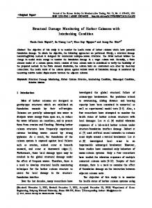
Thus the inverse identification problem consists of finding the system inputs from the dynamic responses, boundary conditions and a system model. The different methods for identifying structural loads can be categorized into deterministic methods, stochastic methods, and methods based on artificial intelligence. A review of methods for force reconstruction is given by Uhl (2007). Since monitoring wind turbines typically concerns the operational phase, the reconstruction of forces is of secondary interest. In turn, more stress must be focussed on determining the residual life time of a structure. Determining the residual life time is based on the evaluation of cyclic loads. Structures errected in the field are typically subjected to cyclic loads resulting from ambient excitation such as wind or wave loads in the case of off-shore wind turbines or traffic loads for bridges. A cyclic sinusoidal load is characterized by three specifications. Two specifications define the load level, e.g. maximum stress Smax and minimum stress Smin or mean stress Sm and stress amplitude Sa . The third specification is the number of load cycles N. Depending on the stress ratio R = Smin /Smax , the cyclic load can be divided into the following cases: pulsating compression load, alternating load, pulsating tensile load or static load, and into intermediate tensile/compressive alternating load (Haibach, 2006). A measure for the capacity of a structural component to withstand cyclic loads with constant amplitude and constant mean value is given by its S/N-curve, also reffered to as Wöhler curve, Fig. 2. Basically, the S/N-curve reveals the number of load cycles a component can withstand under continuous or frequently repeated pulsating loads (DIN 50 100, 1978). Three levels of endurance characterize the structural durability: low-cycle, high-cycle or finite-life fatigue strength and the ultra-high cycle fatigue strength. The endurance strength corresponds to the maximum stress amplitude Sa and a given mean stress Sm which a structure can withstand when applied arbitrarily often (DIN 50 100, 1978) or more frequent than a technically reasonable, relatively large number of cycles. However, the existence of an endurance strength is contentious issue, since it has been demonstrated that component failures are also caused in the high-cycle regime (Sonsino, 2005). The transition to finite-life fatigue strength is characterized by a steep increase of the fatigue strength. The knee-point, which seperates the long-life and the finite-life fatigue strength corresponds to a cycle number of about ND = 106 − 107 . Both, long-life and finite-life fatigue strength are dominated by elastic strains. In contrast to this, low-cycle fatigue strength is dominated by plastic strains. The transition from finite-life to low-cycle fatigue strength is in the area of the yield stress (Radaj, 2003). S/N-curves are derived from cyclic loading tests. The tests are carried out on unnotched or notched specimens or on component-like specimens. Load profiles applied to the specimen are either axial, bending or torsional. To derive one curve, the mean stress Sm or the minimum stress Smin is left constant for all specimens, only the stress amplitude Sa or maximum stress Smax is modified. The numbers of load cycles a specimen withstands up to a specific failure criterion, e.g. rupture or a certain stiffness reduction, is plotted horizontaly against the corresponding stress amplitude values (DIN 50 100, 1978; Radaj, 2003). The previous considerations concern the durability of structures subjected to constant amplitude loading. However, most structures under operational conditions experience loading environments with variable mean loads and load amplitudes. This differentiation is important since fatigue response may be very sensitve to the specifics of the loading type (Heuler & Klätschke, 2005).

www.intechopen.com

210 4

Fundamental and Advanced Topics Will-be-set-by-IN-TECH in Wind Power

stress

Smax

Sm time

Smin

Sm

Smin

rel. frequency of occurance

number of cycles N

finite-life fatigue

long-life fatigue

Smax

Sm time

stress

Smax

stress

stress amplitude Sa (log)

yield point

stress

Smax

low-cycle fatigue

Sm

knee point Smin

Smin

ND numbers of cycles N(log)

rel. frequency of occurance

Fig. 2. S/N-curve.

Fig. 3. Load spectra derived by level crossing counting from constant and variable amplitude load-time histories, after Haibach (1971).

The fatigue life curve, or: Gassner curve, is determined in similar tests but using defined sequences of variable amplitude loads (Sonsino, 2004). Depending on the composition of the load spectrum, the fatigue life curve deviates from the S/N-curve. The relation between both curves is represented by a spectrum shape factor (Heuler & Klätschke, 2005). The content of a variable load time history, e.g. the relative frequency of occurance of each amplitude, can be illustrated in a load spectrum. Different cycle counting methods exist to derive load spectra. An overview of the so called one-parameter counting methods is given in DIN 45 667 (1969) and Westermann-Friedrich & Zenner (1988). Level crossing and range-pair counting are historically well established one-parameter counting methods (Sonsino, 2004). As an example Fig. 3 shows load spectra derived from constant amplitude and variable amplitude load-time-history. The mean stress Sm and the maximum stress amplitude Smax is common to the resulting load spectra. However, the constant amplitude load spectrum reveals a high cycle number for the maximum amplitude, while the variable amplitude load spectrum reveals high cycle numbers only for smaller amplitudes. Fig. 4 shows examples of load spectra. In general, the fuller a load spectrum is, i.e. the more relatively large amplitudes it contains, the less load cycles a structure withstands without damage, Fig. 4 (Haibach, 2006). From today’s perspective, most of the one-parameter counting methods can be considered as special cases of the two-parameter rainflow counting method (Haibach, 2006). The rainflow load spectrum shape

SA

stress amplitude SA [N/mm2]

SA,1

S/N-curve SA,2

400

200

SA,n

100

n1 50 103

104

105

106

107

108

number of cycles N

Fig. 4. Effect of different load spectra on the fatigue life curve, after Haibach (2006).

www.intechopen.com

n2

ni

109

N N1

N2

Fig. 5. Load spectrum and S/N-curve.

Ni

Monitoring andDetection Damage Detection inTurbines Structural Parts of Wind Turbines Monitoring and Damage in Structural Parts of Wind

2115

counting method is the most recent and possibly the most widely accepted procedure for load cycle counting (Boller & Buderath, 2006). Each loading cycle can be defined as a closed hysteresis loop along the stress-strain path. The maximum and the mininum values or the amplitude and the mean values of the closed hysteresis loops are charted as elements into the rainflow matrix. Rainflow matrices allow distribution of the hysteresis loops to be determined. A detailed description of the method is given by Haibach (2006), Radaj (2003) and Westermann-Friedrich & Zenner (1988). In order to provide representative load data, standardized load-spectra and load-time histories (SLH) have been previously be developed. SLH are currently available for various fields of application such as in the aircraft industry, automotive applications, steel mill drives, as well as for wind turbines and off-shore structures. In particular, the SLH WISPER/WISPERX (Have, 1992) and WashI (Schütz et al., 1989) exist for wind turbines and off-shore structures, respectively (Heuler & Klätschke, 2005). The residual life time of a component is estimated by means of a damage accumulation hypothesis. For this reason, a load spectrum for the specific component, a description of the stress concentration for notches in the component and an appropriate fatigue life curve are required (Boller & Buderath, 2006). Within numerous damage accumulation hypotheses the linear hypothesis of Palmgren and Miner plays an important role in practical applications. Different modifications of the hypothesis exist. Basically, the idea of the hypothesis is to determine the residual life time of a component via the sum of the load cycles which the component experiences in relation to its corresponding fatigue life curve, Fig. 5. A partial damage D j is calculated for a certain load amplitude S j with Dj =

ΔNj NFj

,

(2)

where ΔNj is the number of load cycles corresponding to S j and NFj is the number of load cycles with the same load amplitude corresponding to the fatigue failure curve, up to failure. The total damage D resulting from the load cycles of different load amplitudes S j with j = 1, 2, ..., n is yielded by: n

D=

∑ Dj .

(3)

j =1

According to the hypothesis the component fails when its total damage attaines unity, D = 1. However, several studies demonstrate that in particular cases, the real total damage may deviate significantly from unity. Prerequestives for the right choice of the S/N-curve are that the material, the surface conditions, the specimen geometry and loading conditions are appropriate (Radaj, 2003). 2.2 System description

To measure the operational loading, strain gauges are applied to the structure’s hot spots determined during the development phase. The strain gauges can be connected to smart sensor nodes placed adjacent to the spots (see Fig. 6). Running a rainflow counting algorithm on the smart sensor nodes yields an analysis of the real operational loads the structure is subjected to. Due to the data reduction using the rainflow counting, the amount of data to be transmitted to a central unit is reduced to a minimum. Furthermore, the data are only transmitted when an update of the residual life time is requested by the operator (e.g. every 10 minutes).

www.intechopen.com

212 6

Fundamental and Advanced Topics Will-be-set-by-IN-TECH in Wind Power

strain gauge 1 connected to smart sensor node 1 strain gauge 2 connected to smart sensor node 2

strain gauge n connected to smart sensor node n

Fig. 6. Load Monitoring system based on decentralized preprocessing with smart sensor nodes. Using the load spectra as input, damage accumulation is calculated on the central unit (see Fig. 6 for the connection scheme of smart sensor nodes and the central unit). Next, the residual life time can be determined by comparing those damage accumulation with the endurable loading. Furthermore, with this Load Monitoring concept, exceptional loads can be determined and used to trigger analyses of the structure’s integrity using other monitoring methods. 2.3 Application: Model of a wind turbine

To test the performance of the decentralized Load Monitoring in the field, a structure is chosen which is exposed to actual environmental excitations by wind loads. A small model of a wind turbine (weight approx. 0.5 kg) is mounted on top of an aluminum beam, which serves as a model for the tower (see Fig. 7). Although quite simple and small, the wind turbine model possesses a gearbox with several stages which may serve as a potential noise source during operation. For a test, the beam is instrumented with four strain gauges which are wired to a Wheatstone bridge and mounted close to the bottom of the beam as shown in Fig. 7. The left side of Fig. 8 shows a rainflow matrix calculated under wind excitation and the associated damage accumulation. The implementation has been conducted to the effect, that the smart sensor node determines the turning points from the strain signal before calculating the rainflow matrix by using the rainflow counting algorithm. Following this, the rainflow matrix was periodically (in this case every 10 minutes) sent to a central unit. By means of this, the communication effort and the real time requirements between the two participants in network have been reduced. Based on the data-update, the central unit (a desktop PC in this case) estimates the current damage accumulation. The result of this is a damage accumulation function growing over time steps of 10 minutes, as shown on the right side of Fig. 8. The function rises slowly, caused by a small number of load cycles or a minor strain signal amplitude. In contrast to this, the steep rising at about t = 200 min, is due to a large number of load cycles or a large strain amplitude, as the case may be. The Palmgren-Miner rule states that failure occurs when the value of the accumulate damage is unity. In this test, with only a wind loading measured over a period of 220 minutes, the calculated damage accumulation is remote from this critical value.

www.intechopen.com

2137

Monitoring andDetection Damage Detection inTurbines Structural Parts of Wind Turbines Monitoring and Damage in Structural Parts of Wind

1350

Wind turbine model

Tower model (aluminum beam) 15

Strain gauge

20

Y

Y X

100

Z

(a)

X

S1

(b)

Fig. 7. Experimental set-up. (a) A model of a wind turbine was exposed to actual environmental excitations by wind loads on the top of a building. (b) Strain gauges were mounted nearly at the bottom of the beam.

max

damage sum

Rainflow-Matrix t = 220 min

min

time [min]

Fig. 8. Left: A matrix calculated under wind excitation. Right: The damage accumulation growing over time.

3. Vibration analysis 3.1 Basic principles

The process of monitoring the health state of a structure involves the observation of a system over time by the means of dynamic response measurements, the extraction of damage-sensitive features from these measurements, and the statistical analysis of these features. Features are damage sensitive properties of a structure which allow difference between the undamaged and the damaged structure to be distinguished (Sohn et al., 2004).

www.intechopen.com

214 8

Fundamental and Advanced Topics Will-be-set-by-IN-TECH in Wind Power

Some vibration-based damage sensitive properties are described in the following. Resonant frequencies. Monitoring methods based on resonant frequencies can be categorized into the forward and the inverse problem. The forward problem consists of determining frequency shifts due to known damage cases. Damage cases are typically simulated using numerical models. Damages can then be identified by comparing the simulated to the experimentally measured frequencies. The inverse problem consists in determining damage parameters from shifts in resonant frequencies. However, the major drawback of monitoring methods based on frequency shifts is the low sensitivity of resonant frequencies to damage (Montalvão et al., 2006). Mode shapes. Using mode shapes as a feature for damage detection is advantageous over using methods based on resonant frequencies since mode shapes contain local information about a structure which makes them sensitive to local damage. This is a major advantage over resonant frequencies which are global parameters and thus can only detect global damage. Furthermore, mode shapes are less sensitive to environmental effects such as temperature. ’Traditional mode shape change methods’ are based on damage identification from mode shape changes which are deteremined by comparing them to finite element models or preliminary experimental tests. On the other hand, ’modern signal processing methods’ can be applied alone to actual mode shape data from the damaged structure. Here, the damage location can be revealed by detecting the local disconinuity of a mode shape. A promissing feature of enhancing the damage sensitivity of mode shape data is the use of mode shape curvatures. A curvature is the second derivative of a mode shape. The modal strain energy-based methods can be considered as a special case of the curvature-based method. The method uses changes of fractional modal strain energies, which are directly related to mode shape curvatures. Within the modal strain energy-based methods particular attention is paid to the damage index method (DIM) (Fan & Qiao, 2010). Frequency domain response functions. The use of non-modal frequency domain response functions for monitoring can be advantageous over modal-based methods. In contrast to response functions modal parameters are indirectly measured. Thus they can be falsified by measurement errors and modal extraction faults. Further, the completeness of modal data can not be guaranteed in most practical applications because a large number of sensors is required (Lee & Shin, 2001). One approach to detecting the damage locations on complex structures using directly measured frequency-domain response functions is based on the Transmissibility Function (TF) (Siebel & Mayer, 2011). The TF for one element of a structure is built from the ratio of the response functions of two adjacent points. TFs can be calculated from system outputs without knowing the exact input forces. Hence, in order to apply the method, information about the source of excitation is not neccessarily required (Chesné & Deraemaeker, 2010). In the technical literature, the topic of feature extraction has received much attention. Reviews and case studies have been written by Sohn et al. (2004), Carden & Fanning (2004), Montalvão et al. (2006), Humar et al. (2006), Fan & Qiao (2010) and, with special emphasis on the monitoring of wind turbines, by Ciang et al. (2008) and Hameed et al. (2007). The large size of wind turbines and the difficult accessibility complicates maintenance and repair work. Thus, in order to guarantee safety and to improve availability, the implementation of an autonomous monitoring system that regularly delivers data about the

www.intechopen.com

Monitoring andDetection Damage Detection inTurbines Structural Parts of Wind Turbines Monitoring and Damage in Structural Parts of Wind

2159

structural health is of practical interest. Furthermore, easy handling and installation, i.e. low cabling effort, are required for practicability. The implementation of vibration-based monitoring methods requires frequency or modal data. Modal data of real structures can be extracted by methods of system identification. The demands for autonomy of the montitoring system and for a regular data transfer makes system identification a challenging task. That is, because vibration must be measured under operating conditions and no defined force is applied. On off-shore wind turbines, vibration is induced into the structure by ambient excitation, e.g. by wind or wave loads. System identification methods handling these conditions are referred to as output-only system identification methods, in-operation or as Operational Modal Analysis (OMA). Important output-only system identification methods for the extraction of modal data (i.e. natural frequency, damping ratio and mode shapes) are outlined below. The first four categories of methods presented are based on time-domain responses, whereas the methods of the last category use frequency-domain responses. NExT. Traditional time domain multi-input multi-output (MIMO) Experimental Modal Analysis (EMA) uses impulse response functions (IRF) to extract modal parameters. The Natural Excitation Technique (NExT) adopts the EMA methodology by employing Correlation Functions (COR) instead of IRF. COR can be obtained by different techniques such as the Random Decrement (RD) technique, inverse Fourier Transform of the Auto Spectral Density, or by direct estimates from the random response of a structure subjected to broadband natural excitation. Both COR and IRF are time domain response functions that can be expressed as sum of exponentially-decayed sinusoidals. The modal parameters of each decaying sinusoidal are identical to those of the corresponding structural mode (Zhang, 2004). ARMA. The dynamic properties of a system in the time domain can be described by an Auto-Regressive Moving Average (ARMA) model. In the case of a multivariate system, the model is called Auto-Regressive Moving-Average Vector (ARMAV) (Andersen, 1997). The parametric ARMAV model describes the relation of the system’s responses to stationary zero-mean Gaussian white noise input and to AR (auto-regressive) and MA (moving-average) matrices. The AR component describes the system dynamics on the basis of the response history and the MA component regards the effect of external noise and the white noise excitation. The ARMAV model can be expressed in the state-space from which natural frequencies, damping ratios and mode shapes can be extracted (Bodeux & Colinval, 2001). A number of algorithms for the Prediction-Error Method (PEM) have been proposed in order to identify modal parameters from ARMAV models. However, the PEM-ARMAV type OMA procedures have the drawback of being computationally intensive and of requiring an initial ’guess’ for the parameters which are to be identified (Zhang et al., 2005). Covariance-driven SSI. The covariance-driven Stochastic Subspace Identification (SSI) methods allows state-space models to be estimated from measured vibration data. For system realization, measured impulse response or covariance data are used to define a Hankel matrix. The Hankel matrix can be factorized into the observability matrix and the controllability matrix. The system matrices of the state-space model can then be extracted from the observability and the controllability matrices. Various SSI methods have been developed for the system realization, e.g. Principal Component (PC) method,

www.intechopen.com

216 10

Fundamental and Advanced Topics Will-be-set-by-IN-TECH in Wind Power

Canonical Variant Analysis (CVA) and Un-weighted Principal Component (UPC) method. The methods differ in the way the observability matrix is estimated, and also in how it is used for finding the system matrices. The last step of the stochastic realization-based OMA is the calculation of the modal parameters from the system matrices. These methods are also referred to as stochastic realization-based procedures (Viberg, 1995; Zhang et al., 2005). Data-driven SSI. The advantage of the data-driven over the covariance-driven SSI is that it makes direct use of stochastic response data without an estimation of covariance as the first step. Furthermore, it is not restricted to white noise excitation, as is the covariance-driven SSI, but it can also be employed for colored noise. The data-driven SSI predicts the future system response from the past output data. Making use of state prediction leads to a Kalman filter for a linear time-invariant system. It can be expressed by a so-called innovation state-space equation model, where the state vector is substituted by its prediction and where the two inputs (i.e. process noise and measurement noise) are converted to an input process – the innovations. After computing the projection of the row space of the future outputs on the row space of the past outputs and estimating a Kalman filter state, the modal parameters are calculated as before with UPC, PC or CVA (Andersen & Brincker, 2000; Zhang et al., 2005). Frequency Domain Decomposition. The classical frequency-domain approach for OMA is the Peak Picking (PP) technique. Modal frequencies can be directly obtained from the peaks of the Auto Spectral Density (ASD) plot, the mode shapes can be extracted from the column of the ASD matrix which corresponds to the same frequency. The PP method gives reasonable estimates of the modes, it is fast and simple to use. However, PP can be inaccurate when applied to complex structures, especially in the case of closely spaced modes. The Frequency Domain Decomposition (FDD) is an extension of PP which aims to overcome this disadvantage. The FDD technique estimates modes from spectral density matrices by applying a Singular Value Decomposition. This corresponds to a single-degree-of-freedom identification of the system for each singular value. The modal frequencies can then be obtained from the singular values and the singular vectors are an estimation of the corresponding mode shapes. The Enhanced Frequency Domain Decomposition (EFDD) is a further development of the FDD. In addition to modal frequencies and shapes, the EFDD can estimate modal damping. For this, singular value data is transferred to time-domain by an inverse Fourier transformation. Modal damping can then be estimated from the free decay (Herlufsen et al., 2005; Zhang et al., 2005). 3.2 System description

The system presented here is designed to autonomously acquire the development of the modal properties of the system under test. In this, it just delivers data useable for Structural Health Monitoring (SHM), but it does not autonomously carry out analyses of them. The system accounts for the requirements mentioned above in the following way: To satisfy the demand for autonomy and to be able to use ambient instead of artificial excitation, the measured data is analysed using the algorithms of OMA. To lower the cabling effort, a network of smart sensors is designed in which the sensor nodes are capable of preprocessing the data using the RD method. Due to the reduction of the amount of data to be transmitted, the sensor nodes can be connected in a bus structure with the central processing unit. The microcontrollers usually applied in (wireless) sensor platforms are typically not capable of performing extensive computations. For instance, only basic calculations like spectral

www.intechopen.com

Monitoring andDetection Damage Detection inTurbines Structural Parts of Wind Turbines Monitoring and Damage in Structural Parts of Wind

217 11

estimation of the acquired data sequences can be implemented (Lynch et al., 2006). In this paper, the RD method is evaluated with respect to distributed signal processing on sensor nodes. It is a simple, yet effective method for estimating correlation functions (Brincker et al., 1991; Cole, 1973), and was originally devised for detecting damage in aerospace structures subjected to random loading. It can also successfully be applied as a component of a structural parameter identification, e.g. in OMA (Asmussen, 1998; Rodrigues & Brincker, 2005). Having estimated averaged correlation functions by means of the smart sensors, these functions are transferred to a central processing unit. There, the algorithms of Frequency Domain Decomposition (FDD) are applied to estimate the eigenfrequencies and mode shapes of the system under test. 3.2.1 Description of the Random Decrement technique

As mentioned above, most of the parts of a wind turbine being of interest to SHM cannot be artificially excited for structural analyses, because they might be too large (e.g. the whole tower) or because it is impractical to apply a vibration exciter during its operation. Thus only the output signals, i.e. the vibrations excited by operational loads can be used in order to estimate the system’s behavior. Extracting this information can be done using the RD method, which is a simple technique that averages time data series x (tn ) measured on the system under random input loads when a given trigger condition is fulfilled (see Equation 4 as an example of a level crossing trigger at trigger level a). The result of this averaging process from n = 1 to N is called an RD signature DXX (τ ).   1 N  (4) x (tn + τ ) x (tn ) = a DXX (τ ) = ∑  N n =1

The method can be explained descriptively in the following way: At each time instant, the response of the system is composed of three parts: The response to an initial displacement, the response to an initial velocity and the response to the random input loads during the time period between the initial state and the time instant of interest (Rodrigues & Brincker, 2005). By averaging many of those time series, the random part will disappear, while the result can be interpreted as the system’s response to the inital condition defined by the trigger, thus, containing information about the system’s behavior. A depictive example can be found in Friedmann et al. (2010). Asmussen (1998) proved that a connection between RD signatures DXX and correlation functions R XX can be established. For a level crossing trigger conditon, the factors used to derive correlation functions from RD signatures are the trigger level a itself and the variance σx2 of the signal triggered (see Equation 5). σx2 (5) a These factors can be derived from the measurements without incurring high computational or memory costs so that the estimation of correlation functions can be implemented in a decentralized network of smart sensors. The concept may be extended from autocorrelation functions as described above to the estimation of cross-correlation functions between two system outputs. This is simply achieved by averaging time blocks from one system output (here y) while the averaging process is triggered by another output (here x). If a simple level crossing trigger is assumed, the mathematical expression of the RD technique as established by Asmussen (1998) is: R XX (τ ) = DXX (τ )

www.intechopen.com

218 12

Fundamental and Advanced Topics Will-be-set-by-IN-TECH in Wind Power

  1 N  y(tn + τ ) x (tn ) = a. (6) DYX (τ ) = ∑  N n =1 The conversion of a cross RD signature to a cross-correlation function is expressed by Equation 7. RYX (τ ) = DYX (τ )

σx2 a

(7)

3.2.2 Description of Operational Modal Analysis based on the Random Decrement method

The idea behind the described data acquisition system is to estimate RD signatures by the smart sensors and to transfer them to a central unit. On this central unit, the correlation functions are calculated and the modal analysis is performed. In the application described here, this central unit is a common desktop computer where the matrices R of the correlation functions are evaluated by a Matlab routine. Having calculated all correlation functions of the matrix R, an intermediate step is needed before starting with the modal decomposition. Because the algorithms of frequency domain based OMA need a matrix G(f) of spectral densities as an input, a single block Discrete Fourier Transform (DFT) has to be applied to the correlation functions (McConnell, 1995). It should be mentioned that within this DFT, no use is made of time windowing. For the subsequent OMA, the FDD algorithm is used. This algorithm, first described by Brincker et al. (2000), is based on a Singular Value Decomposition of the matrix G(f). For every frequency f , this process leads to two fully populated matrices U(f) and a diagonal matrix S(f) holding the spectra of the so-called singular values Sii ( f ) in decreasing order (see Equation 8). G (f) = U (f) S (f) UH (f)

(8)

The peak values of the first singular values are then interpreted as indicators for the systems’ eigenfrequencies. Furthermore, using the FDD algorithm, it is possible to estimate the mode shapes for the found frequencies. The eigenvectors describing the mode shapes corresponding to the eigenfrequencies determined by the spectra of the singular values can be found in the corresponding columns of the matrix U(f). Performing an OMA in the usual way, picking the peaks from the spectra of the singular values Sii ( f ), requires users’ input. However, because the modal decomposition has to be automated for the use in SHM, the need for such users’ input must be eliminated. Therefore, an algorithm is needed that is able to pick the spectral peaks in a similar way to an educated user. Much work has been done in this area and some solutions are implemented in commercial software, e.g. by Peeters et al. (2006), Andersen et al. (2007), and Zimmerman et al. (2008). In the implementation used here, an algorithm is employed for the peak picking that only operates using the numerical data of the given spectra. In doing so, the numerical data of the given spectra is analyzed automatically for potential eigenfrequencies. The procedure regards three parameters, a lower noise threshold, an upper signal bound and a value for the sensitivity in the frequency dimension. The sensitivity enables a residual random part of peaks in the spectra to be eliminated which are due to the finite number of averages used to calculate the RD signatures RYX (τ ).

www.intechopen.com

Monitoring andDetection Damage Detection inTurbines Structural Parts of Wind Turbines Monitoring and Damage in Structural Parts of Wind

219 13

3.3 Applications 3.3.1 Model of a wind turbine

To test the performance of the vibration analysis approach in the field, the model of a wind turbine described in Section 2.3 is used. The cross-section and length of the beam serving as the tower are appropriately chosen, such that the resonant frequencies of the assembled system are in a range similar to those of a full scale structure. Since the cross-section of the beam is rectangular, the bending eigenmodes in the x and y directions should possess different eigenfrequencies in order to alleviate the structural analysis. For the tests, the beam is instrumented with two triaxial, laboratory accelerometers with a sensitivity of 0.1 V/g and a measuring range of ±50 g. One sensor is mounted close to the top of the beam (sensor 1) and the other mid-way along the length (sensor 2). In this first application, only the x-axis is used for data acquisition using the network described. As a reference for the measurements under operating conditions, an EMA and an OMA are conducted. The results of those analyses (first bending modes around 4.5 Hz, second bending modes around 30.0 Hz) are listed and compared to other results in Table 1. For the OMA, the commercial software ARTeMIS has been used. It has to be mentioned that for the first and the second bending modes the frequency in the x and y directions fit each other even though the aluminum beam has no quadratic cross-section. This can be explained with the asymmetric fixture at the lower end of the beam. Both sensor signals are processed on one hardware platform but by means of a decentralized implementation. This is considered as a first step for functional prototyping of the algorithms and the system layout in general. The estimation of the RD signatures follows Equation 4 and Equation 6. The estimation of the signal’s variance σx2 is done using an autoregressive power estimator (Kuo & Morgan, 1996). Its implementation requires only one storage bin and its use is possible due to the fact that signals without zero mean (as is the case with the used accelerations), the signals’ power or mean square value equals the variance (Bendat & Piersol, 2000). A sampling rate of 200 Hz was chosen, which is high enough to acquire vibrations related to the first few bending modes. The RD signatures’ length was set to 1000 elements; the signatures shown are averaged 8192 times. The estimated RD signatures DYX are shown in Fig. 9. A comparison of the cross-correlation functions R11 and R22 is shown in Fig. 10 to check that the assumption of reciprocity holds like it should be for every mechanical system. The matrix of spectral densities G(f) derived from the correlation functions is shown in Fig. 11 and the peaks selected by the peak picking algorithm are marked by circles in Fig. 12. The results are the same as an educated user would have guesstimated. Only the peak at 50 Hz found within the experimental set-up would not have been chosen by a user because it clearly originates from a power line pickup. The eigenfrequencies found for the experimental set-up are 4.2 Hz and 33.4 Hz, respectively. Those results deviate max. ± 6% from the frequencies calculated or measured directly (see Table 1). mode measured by EMA 1. 2.

4.3 Hz / 4.4 Hz 31.6 Hz / 29.7 Hz

estimated by FDD in estimated with the ARTeMIS network described here 4.2 Hz / 4.4 Hz 4.2 Hz / y not estimated 31.5 Hz / 29.0 Hz 33.4 Hz / y not estimated

Table 1. Comparison of eigenfrequencies (x-axis / y-axis) measured for the wind turbine using different approaches.

www.intechopen.com

220 14

Fundamental and Advanced Topics Will-be-set-by-IN-TECH in Wind Power

−4

−4

[g]

x 10 12

5

RD signature D

RD signature D

11

[g]

x 10

0 −5 0

5

0 −5

2 4 time τ [s]

0

−4

−4

[g]

x 10 22

5

RD signature D

21

[g]

x 10 RD signature D

2 4 time τ [s]

0 −5 0

5

0 −5

2 4 time τ [s]

0

2 4 time τ [s]

Fig. 9. Matrix D of the RD signatures measured on the model of a wind turbine.

−4

1.5

x 10

cross−correlation R12 cross−correlation R

21

cross−correlation R

YX

2

[g ]

1

0.5

0

−0.5

−1

−1.5

0

1

2 time τ [s]

3

4

Fig. 10. Comparison of cross-correlation functions R12 and R21 of the wind turbine.

www.intechopen.com

221 15

−5

0 50 frequency [Hz] −5

22

10

G

G

21

[g2/Hz]

[g2/Hz]

0 50 frequency [Hz] 10

0 50 frequency [Hz]

−4

10

2

12

G

G

11

−5

10

singular value [g /Hz]

−5

10

[g2/Hz]

[g2/Hz]

Monitoring andDetection Damage Detection inTurbines Structural Parts of Wind Turbines Monitoring and Damage in Structural Parts of Wind

−6

10

−8

0 50 frequency [Hz]

Fig. 11. Matrix of spectral densities G(f).

10

0

20 40 frequency [Hz]

60

Fig. 12. Spectra of the first (-) and second (- -) singular values S 11 ( f ) and S22 ( f ) of the wind turbine.

3.3.2 Pedestrian bridge

As the first real application for the proposed system, the monitoring of a pedestrian bridge is described. This bridge shown in Fig. 13 connects two buildings and has a length of 20 m. To gain fundamental insight into the behavior of this bridge, an EMA has been performed. From this analysis, the main parameters of the monitoring system have been analytically derived (see Table 2). The steps needed to calculate this parameters are described below.

Fig. 13. North view of the bridge subjected to monitoring. Parameter Symbol Value Frequencies of modes of interest [ f 1 , ..., f HMoI ] [8.1, 9.8, 15.1] Hz Frequency of highest mode of interest f HMoI 15.1 Hz Structural damping loss factor of modes of interest [η1 , ..., η HMoI ] [0.63, 0.43, 1.23] % Xend Desired decay of the sigantures 1% X Sampling frequency fs 128 Hz Block length of RD signatures (in samples) n 2048 Block length of RD signatures (in seconds) T 16 s Table 2. Setup of the monitoring system derived from the EMA.

www.intechopen.com

222 16

Fundamental and Advanced Topics Will-be-set-by-IN-TECH in Wind Power

The first step in defining the setup of the monitoring system from the EMA is to select the range of modes that should be monitored. This selection should be based on the experience of a monitoring engineer as well as on knowledge about the hot spots of the system being monitored. These are given by the user or manufacturer. Having chosen the modes of interest, the sampling frequency and block length can be calculated using the output coming from the EMA as well as some values defined by the user (see Equations 9 and 10). f s = [2...8] · f HMoI

T ≥ max

⎧ ⎪ ⎪ ⎪ ⎨ ⎪ ⎪ ⎪ ⎩





ln XXend η 2π f − 2f  η 2 f 1− 2

 1  T = a  a ∈ 2N fs

⎫   ⎪ ⎪  ⎪ ⎬   f ∈ f , ..., f ] [  HMoI 1  ⎪ ⎪  ⎪ ⎭ 

(9)

(10)

The quality of the determined mode shapes strongly depends on the accuracy of the estimated phase relationships acquired using the cross RD signatures (see Section 3.2.1). Therefore the acquired cross RD signatures should include good quality information about all the modes of interest. This might be archieved by choosing the triggering sensors or reference degrees of freedom (refDOF), in a way that each mode of interest is excitable at least at one refDOF. A similar requirement is described by the controllability criterion of a controlled system. Aiming at optimal controllability, the input matrix of a state-space-model can be used (Lunze, 2010). The state-space-model can be derived from the EMA of the bridge’s structure (Bartel et al., 2010; Buff et al., 2010; Herold, 2003). For monitoring the pedestrian bridge under operating conditions, the signal processing algorithm presented in section 3.2.1 is implemented on an embedded PC by automatic code generation from Simulink. Generally, the resources of the used embedded PC are limited. Based on the PC capacity and the setup parameters, the maximum number of sensors that can be handled by the hardware can be calculated. To guarantee real-time capability, the worst-case sensor-task execution time must be less than the sensor signal’s sampling time. From this it follows that for the bridge application, the hardware can handle a maximum number of 14 sensors (2 reference and 12 response sensors). In contrast, an EMA is usually performed with a huge number of DOFs. Hence, out of these EMA candidate sensor positions, the best possible set of 14 sensor positions has to be chosen. The Effective Independence is a sensor placement method based on the linear independence of candidate sensor sets. In an iterative process, a large starting set is reduced to a given number of 14 sensors (Buff et al., 2010; Kammer, 1991). The second step includes the initialisation of the operational monitoring system on the pedestrian bridge. Prior to starting the data acquisition, the system needs information about the characteristics of the bridge’s natural excitation to determine sensor parameters like sensitivity, resolution and optimum trigger levels for both reference nodes. Therefore the acceleration data of the sensors have been recorded and analysed (see Fig. 14). Two characteristic types of ambient excitations are effective on the bridge: passing pedestrians and wind excitation. √ According to Asmussen (1998), the optimum trigger level is a = 2σx , in the case of the level crossing trigger condition. In the real application it is inappropriate to calculate the standard

www.intechopen.com

223 17

Monitoring andDetection Damage Detection inTurbines Structural Parts of Wind Turbines Monitoring and Damage in Structural Parts of Wind reference 1

reference 2

reference 1

reference 2 0.03

0.1

0.1

0.02

0.02

0.05

0.05

0.01

0.01

0 −0.05 −0.1

0 −0.05 −0.1

0

200

400 t [s]

600

input [m/s2]

0.03

input [m/s2]

0.15

input [m/s2]

input [m/s2]

0.15

0 −0.01 −0.02

0

200

(a)

400 t [s]

−0.03

600

0 −0.01 −0.02

0

200

(b)

400 t [s]

−0.03

600

0

200

(c)

400 t [s]

600

(d)

Fig. 14. At the reference nodes there are two characteristic types of natural excitations on the bridge. (a) pedestrian excitation reference 1; (b) pedestrian excitation reference 2; (c) wind excitation reference 1; (d) wind excitation reference 2. deviation σx from the total sensor signal period, because of the poor signal-to-noise ratio (SNR) due to the measuring hardware over a wide range. For this reason, an experimental trigger level ae has been calculated from only those sections with a sufficient SNR. For the bridge application, this will be the case if a pedestrian passes over the bridge (see Fig. 15). reference 1

reference 2

reference 2

reference 2 0.1

−0.1 0

20 40 t [s] reference 1

−0.1

2

0 −0.05

300 t [s]

0 −0.1

680

700 t [s]

680

0

720

(a)

2

120 140 t [s] reference 2

0.15 0.1

0.05 0 −0.05 −0.1

280

300 t [s]

0 −0.05

100

0.1

−0.05

0.05

−0.1

0.15

0.05

−0.1 700 t [s]

−0.05

720 740 t [s] reference 2

0.1

−0.05

0

20 40 t [s] reference 2

0.15

0.05

0.05

−0.1 0

0.1

0.05

−0.1 280

−0.05 −0.1

0.15 input [m/s ]

input [m/s2]

0

0

120 140 t [s] reference 1

0.1

−0.05

0.05

100

0.15

0.1 0.05

−0.05 −0.1

720 740 t [s] reference 1

0.15

0

2

−0.05

0.05

input [m/s ]

0

input [m/s2]

−0.05

0.05

input [m/s2]

0

2

0.05

input [m/s ]

0.15

0.1 input [m/s2]

0.15

0.1 input [m/s2]

0.15

0.1 input [m/s ]

0.15

0.1

−0.1

input [m/s2]

reference 1

0.15

0.1 input [m/s2]

input [m/s2]

reference 1 0.15

0.05 0 −0.05 −0.1

680

700 t [s]

680

700 t [s]

720

(b)

Fig. 15. If a pedestrian passes over the bridge, the signal-to-noise ratio of the reference sensor signals is sufficient to calculate the experimental trigger levels. (a) signal sections of reference 1 to calculate ae,1 ; (b) signal sections of reference 2 to calculate ae,2 . Consequently, the experimental trigger levels can be calculated as follows: ae,i =

√

2 N σk N k∑ =1

(11)

Having finished the preprocessing and setup up of the smart sensor network, the first measurements were conducted using the 14 DOFs as described. Those measurements yielded consecutive sets of 28 RD signatures. Using the two trigger levels and the two variances acquired together with those signatures, consecutive sets of 28 correlation functions have been calculated and transformed into spectral density matrices. For two correlation functions a reciprocity check could be made. This yielded a good agreement in amplitude and position of the zero crossings. Decomposing these matrices into singular value spectra and using the

www.intechopen.com

224 18

Fundamental and Advanced Topics Will-be-set-by-IN-TECH in Wind Power

10

10

5

5

z [m]

z [m]

peak picking algorithm, the time-dependent development of several eigenfrequencies can be derived. Furthermore, clear mode shapes could be derived from the measured data. Fig. 16 shows a torsional mode of the bridge’s deck. The mode shape and the frequency showed excellent agreement to the shapes and frequencies derived from the EMA.

0 −5

0 0 5 y [m]

15

10

z [m]

x [m]

5

x [m]

5 10

5 0 −5

15 −5

10

0

5

0

5

y [m]

5 10 15 x [m]

y [m] Fig. 16. Mode shape of a torsional mode of the bridge’s deck.

4. Acousto Ultrasonics 4.1 Basic principles

Damage detection methods based on ultrasonics rely on the propagation and reflection of elastic waves within a material. The purpose is to identify local damage and flaws via wave field disturbances (Giurgiutiu & Cuc, 2005). For ultrasound non-destructive evaluation (NDE) a transmitter transfers ultrasound waves into a material and a receiver picks up the waves when they have passed through the material. Transmitter and receiver can be combined into a single component (Lading et al., 2002). Embedding piezoelectric transducers into a structure allows methods for active Structural Health Monitoring (SHM) to be implemented. Piezoelectric transducers are inexpensive, lightweight and unobtrusive and, due to these properties, appropriate for embedding into a structure with minimal weight penalty and at affordable costs. Compared to conventional NDE ultrasound transducers, active piezoelectric transducers interact with a structure in a similar way. One piezoelectric transducer can act as both transmitter and receiver of ultrasonic waves (Giurgiutiu & Cuc, 2005). Among the different types of elastic waves that can propagate in materials, the class of the guided waves plays an important role for SHM. The advantage of guided waves is, that they can travel large distances in structures; even in curved structures, with only little energy

www.intechopen.com

Monitoring andDetection Damage Detection inTurbines Structural Parts of Wind Turbines Monitoring and Damage in Structural Parts of Wind

225 19

loss. Guided waves are being used for the detection of cracks, inclusions, and disbondings in metallic and composite structures. Lamb waves, which are a type of guided wave, are appropriate for thin plates and shell structures. Due to their variable mode structure, multi-mode character, sensitivity to different types of flaws, their ability to propagate over long distances, their capability of following curvatures and accessing concealed components, the guided Lamb waves offer an improved inspection potential over other ultrasonic methods. Another type of guided waves are Rayleigh waves, which travel close to the surface with very little penetration into the depth of a solid, and therefore are more useful for detecting surface defects (Giurgiutiu, 2008). Lamb waves are guided by the two parallel free boundary surfaces of a material. They propagate perpendicularly to the plate thickness. The boundary surfaces only impose low damping to the Lamb waves, thus they can travel long distances. Lamb waves are interesting from the monitoring point of view since damage such as boundary, material or geometric discontinuities which generate wave reflections can be detected (Silva et al., 2010). The Lamb waves can be classified into symmetrical and anti-symmetrical wave shapes, Fig. 17, both satisfying the wave equation and boundary conditions for this problem. Each wave shape can propagate independently of the other (Kessler et al., 2002). Piezoelectric transducers interact with a structure in a similar way to that of conventional ultrasonic transducers. Hence, methods used in traditional ultrasonic monitoring, like pitch-catch or pulse-echo, can be adopted to the application of piezoelectric transducers. The pitch-catch method can be used to detect damage which is located between a transmitter and a receiver transducer. Lamb waves travelling through the damaged region undergo changes in amplitude, phase, dispersion or time of transit. The changes can be identified by comparing with a ’pristine’ situation. The pulse-echo method is based on a single transducer attached to a structure. The transducer functions as both transmitter and receiver of waves. The transducer sends out a Lamb wave which is reflected by a crack. The reflected wave (the echo) is then captured by the same transducer. In contrast to conventional pulse-echo testing where testing is traditionally applied across-the-thickness, the guided wave pulse-echo is more appropriate to cover a wide sensing area. Further ultrasonic approaches for damage detection, which are not detailed, are time reversal methods or migration techniques (Giurgiutiu, 2008). Another technique for acousto-ultrasonic testing is referred to as electro-mechanical impedance method (EMI). Pioneering work on the use of EMI has been carried out by Liang et al. (1994). Only a single piezo transducer is required for its implementation. The technique is based on the direct relation between the electrical impedance (or admittance), which can be measured at the piezo transducers by commercially available impedance analysers, and the

Fig. 17. Graphical representation of anti-symmetrical and symmetrical wave shapes (Kessler et al., 2002).

www.intechopen.com

226 20

Fundamental and Advanced Topics Will-be-set-by-IN-TECH in Wind Power

mechanical impedance of the host structure. The real part of the complex electrical admittance plotted over a sufficiently high frequency range, typically of the order of kHz, is called the ’signature’ of the structure (Ballah & Soh, 2003). Since the imaginary part is more sensitive to temperature variations than the real part, the real part is mainly being used for monitoring applications. In order to achieve high sensitivity to minor changes in the structural integrity the electrical impedance is measured at high frequency ranges of 30-400 kHz. For the choice of the frequency range for a given structure, which is commonly determined by trial-and-error, it must be taken into account that at high frequencies, the sensing area is limited adjacent to the piezoeletric transducer. Estimates of the sensing areas of single PZTs vary anywhere from 0.4 m for composite structures to 2 m for simple metal beams (Park et al., 2003). Furthermore, the modification of a signature increases as the distance between the sensor and the crack decreases (Zagrai & Giurgiutiu, 2002). A comprehensive overview of the topic of SHM with piezoelectric wafer active sensors is given in Giurgiutiu (2008). A method for (passive) SHM, which can be implemented with similar piezoelectric transducer arrangements, is the acoustic emission (AE) method. Sources of acoustic emission within a structure can be cracking, deformation, debonding, delamination, impacts and others. Stress waves of broad spectral content are produced by localized transient changes in stored elastic energy (Ciang et al., 2008). Piezoelectric tranducers can then be used to convert the resulting accelerations into an electric signal. The AE technique allows the growth of damage to be sensed since stress waves are emitted by growing cracks or, in the case of laminates, fibre rupture. Thus the AE technique stands in contrast to many other NDE techniques which generally detect the presence, not the growth of defects. The sensing region of a piezoelectric sensor depends on its particular resonant frequency. For applications to laminates, a common sensor resonant frequency of 150 Hz is a good compromise between noise rejection and the area a sensor monitors (Lading et al., 2002). 4.2 System description and application to carbon fibre reinforced plastic coupons

The method of damage detection with ultrasonic waves should be illustrated by an experimental implementation on a CFRP (carbon fibre reinforced plastic) coupon (Lilov et al., 2010). The aim of the study is to monitor the delamination due to impact damage by acousto-ultrasonic inspection. To this end the coupon is instrumented with two piezo-ceramic transducers (PI 876-SP1). One of them is used as actuator and the other as a sensor (Fig. 18). The test set up (Fig. 19) also includes a dynamic signal analyser, which drives the actuator with a broad band swept sine signal (0..100 kHz), acquires the sensor data and calculates the structural Frequency Response Function (FRF) between actuator and sensor. A PC is connected to the analyser to control the measurements, collect the data and store them for further analysis. To investigate the possibility of determining the severity of the impact event from the measured data, several identical coupons are instrumented and each damaged with a defined impact energy. When directly comparing the measured FRFs from different impact tests, deviations from the original state can be observed (Fig. 20). In order to quantify these effects, a signature based analysis is applied to the FRF. To this end, FRF data Hinit from a reference measurement, i.e. before the damage is induced, is compared to data acquired after the impact event (Hdam ) by calculating statistical measures as damage indices. In many cases, the calculation of the

www.intechopen.com

227 21

Monitoring andDetection Damage Detection inTurbines Structural Parts of Wind Turbines Monitoring and Damage in Structural Parts of Wind

#$%&'%()***+,-'$%*.($'%/(0****1203() *

&,-./-001. !2.3++4

! "###$%%

"!!

&'(

!)*

56('7(-8

!!

Fig. 18. Coupon instrumentation.

!)+

/9,:-8

Fig. 19. Test set up. Frequency Response Function

−20

H [dB]

−40 −60 −80 −100 0

Reference FRF after 40J impact after 10J impact 2

4

6 f [Hz]

8

10 4 x 10

Fig. 20. Frequency response functions before and after different impacts. correlation coefficient leads to good results: Cor ( Hinit , Hdam ) = 

Cov( Hinit , Hdam )  Var ( Hdam )

Var ( Hinit )

(12)

If both measurements lead to identical results, the correlation coefficient value will remain at unity. However, in lower frequency regions, noise from external sources deteriorates the FRF measurements and leads to a low coherence. At very high frequencies, the propagation of ultrasonic waves is damped due to the material properties of the CFRP coupon, this also leads to poor FRF measurements. Thus, it is advisable to choose an expedient frequency band for signature analyses. As shown in Fig. 21, regarding higher impact energies above 15 J, the correlation coefficient decreases with increasing impact energy when analysing the third-octave band around 35.6 kHz. However, for lower impact energies, a deviation of the correlation coefficient from the reference can also be observed. As stated above, this interrelation cannot be observed at a lower frequency band (e.g. 2.8 kHz). Since a broad band excitation is used, and the signals are simply analysed in the frequency domain, a localisation e.g. by time-of-flight analysis is not possible. Thus, this method is more suitable for the straightforward implementation of a damage detection system. Certainly, to transfer this SHM method from the coupon level to an application, some challenges have to be taken up: The system has to be scaled for the application to larger

www.intechopen.com

228 22

Fundamental and Advanced Topics Will-be-set-by-IN-TECH in Wind Power

Correlation Coefficient []

1.5 2,8 kHz band 35,6 kHz band 1

0.5

0 5

10

15

20 25 Impact Energy [J]

30

35

40

Fig. 21. Correlation coefficient for different impacts and frequency bands. components, i.e. several actuator-sensor pairs distributed on the surface. The signal processing should be implemented on a network of smart embedded platforms instead of bulky laboratory equipment. Furthermore, a damage detection algorithm has to be implemented in order to work autonomously. This also includes differentiating between false alarms, e.g. a decrease in correlation due to temperature changes and that from actual impact damage.

5. Conclusions This paper has given an account of the useability of different monitoring methods in wind turbines. The methods described, all serve to supervise of the integrity of structural parts. Different projects have been undertaken at Fraunhofer LBF to develop and evaluate such methods for Structural Health Monitoring, not only in the field of wind energy. This contribution summarizes those developments, starting from the current state of the scientific and technical knowledge and demonstrates their utility for wind turbines with the help of realizations and studies of application of such systems. Three methods have been presented: Load Monitoring, vibration analysis and Acousto Ultrasonics. Concerning Load Monitoring, the development of classical methods for assessing residual life-times and their transfer to smart sensor nodes is presented. As application example, a simple model of a wind turbine is used. The section dealing with vibrational analysis includes a literature review of methods used for extracting health parameters from modal properties as well as the topic Operational Modal Analysis (OMA). The measurement system developed at Fraunhofer LBF makes use of one of those OMA methods and combines it with the Random Decrement method to design a data acquisition system that can be implemented on a smart sensor network. As examples, the application of this system to the model of a wind turbine as well as to a full scale pedestrian bridge is described. As a third method, Acousto Ultrasonics is described as a method which is capable of detecting small scale damages. As an example, its application to coupons of fibre reinforced plastic is described. Although the methods described here are not far enhanced beyond the state of the art documented in literature, their transfer to a network of sensor nodes and especially their capability of being automated is a new and invaluable development deserving discussion. It was demonstrated that, due to their relative small computational effort, all methods possess the potential to be implemented at nodes of smart sensor networks. Their most important

www.intechopen.com

Monitoring andDetection Damage Detection inTurbines Structural Parts of Wind Turbines Monitoring and Damage in Structural Parts of Wind

229 23

limitation lies in the fact that future research will be strongly connected to full scale tests and that such tests cannot be carried out by research organisations alone. Considered as a whole, these results suggest that there are monitoring methods that can be applied to wind turbines and thereby contribute to making the process of harvesting renewable energy more reliable. This research will serve as a base for future studies on the topic of combining the different classes of methods to develop a monitoring system that is able to predict the residual life-time of structures. Such systems are of great use for off-shore wind turbines, because they are the basis of a maintenance on demand.

6. Acknowledgements Parts of the present and still ongoing research in this field as well as the publication of this chapter are funded by the German federal state of Hesse (project „LOEWE-Zentrum AdRIA: Adaptronik Research, Innovation, Application“, grant number III L 4 - 518/14.004 (2008)) as well as in the framework of the programme „Hessen ModellProjekte“ (HA-Projekt-Nr.: 214/09-44). This financial support is gratefully acknowledged.

7. References Andersen, P. (1997). Identification of Civil Engineering Structures using Vector ARMA models, PhD-Thesis, University of Aalborg, Aalborg. Andersen, P. & Brincker, R. (2000). The Stochastic Subspace Identification Techniques, www.svibs.com. Andersen, P., Brincker, R., Goursat, M. & Mevel, L. (2007). Automated Modal Parameter Estimation For Operational Modal Analysis of Large Systems, Proceedings of the 2nd International Operational Modal Analysis Conference, ed. Brincker R. & Møller N., Copenhagen, pp. 299–308. Asmussen, J. C. (1998). Modal Analysis Based on the Random Decrement Technique, Application to Civil Engineering Structures, PhD-Thesis, University of Aalborg, Aalborg. Ballah, S. & Soh, C. K. (2003). Structural impedance based diagnosis by piezo-transducers. Earthquake Engineering and Structural Dynamics, No. 32, pp. 1897-1916. Bartel, T., Atzrodt, H., Herold, S. & Melz, T. (2010). Modelling of an Active Mounted Plate by means of the Superposition of a Rigid Body and an Elastic Model, Proceedings of ISMA2010. International Conference on Noise and Vibration Engineering, pp. 511-523. Bendat, J. S. & Piersol, A. G. (2000). Random Data: Analysis and Measurement Procedures, John Wiley & Sons, New York. Bodeux, J. B. & Colinval, J. C. (2001). Application of ARMAV models to the identification and damage detection of mechanical and civil engineering structures. Smart Materials and Structures, Vol. 10, pp. 479-489. Boller, C. & Buderath, M. (2006). Fatigue in aerostructures – where structural health monitoirng can contribute to a complex subject. Phil. Trans. R. Soc. A, No. 365, Dec 2006. Brincker, R., Krenk, S. & Jensen, J. L. (1991). Estimation Of Correlation Functions By The Random Decrement, Proceedings of The Florence Modal Analysis Conference, Florence, pp. 783–788.

www.intechopen.com

230 24

Fundamental and Advanced Topics Will-be-set-by-IN-TECH in Wind Power

Brincker, R., Zhang, L. & Andersen, P. (2000). Modal Identification from Ambient Response using Frequency Domain Decomposition, Proceedings of the 18th IMAC, San Antonio, TX, USA, pp. 625–630. Buff, H., Friedmann, A., Koch, M., Bartel, T. & Kauba, M. (2011). Systematic preparation of Random Decrement Method based Structural Health Monitoring, Proceedings of the ICEDyn, International Conference on Structural Engineering Dynamics, Tavira, 2011. Accepted for presentation. Carden, E. P. & Fanning, P.(2004). Vibration Based Condition Monitoring: A Review. Structural Health Monitoring, Vol. 3(4), pp. 355–377. Chesné, S.& Deraemaeker, A. (2010). Sur l’utilisation des transmissibilités pour la localisation des défauts dans les systèmes non dispersifs. 10ème Congrès Francais d’Acoustique, Lyon. Ciang, C. C., Lee, J.-R. & Bang, H.-J. (2008). Structural health monitoring for a wind turbine system: a review of damage detection methods. Measurement Science and Technology, No. 19, DOI: 10.1088/0957-0233/19/12/122001. Cole, H. (1973). On-line failure detection and damping measurement of aerospace structures by random decrement signatures, Report NASA CR-2205. DIN 45 667 (1969). Klassierverfahren für das Erfassen regelloser Schwingungen, Beuth-Vertrieb. DIN 50 100 (1978). Dauerschwingversuch – Begriffe, Zeichen, Durchführung, Auswertung, Beuth-Vertrieb. Ewins, D. J. (2000). Modal Testing: Theory, Practice and Application, Research Studies Press, Ltd., Baldock. Fan, W. & Qiao, P. (2010). Vibration-based Damage Identification Methods: A Review and Comparative Study, Structural Health Monitoring, Vol. 10(1), pp. 83-111. Farrar, C. R. & Doebling, S. W. (1997). An Overview of Modal-Based Damage Identification Methods. EUROMECH 365 International Workshop: DAMAS 97, Structural Damage Assessment Using Advanced Signal Processing Procedures. Friedmann, A., Koch, M. & Mayer, D. (2010). Using the Random Decrement Method for the Decentralized Acquisition of Modal Data, Proceedings of ISMA2010. International Conference on Noise and Vibration Engineering, Leuven, September 2010, pp. 3275-3286. Fritzen, C. P., Kraemer, P. & Klinkov, M. (2008). Structural Health Monitoring of Offshore Wind Energy Plants, Proc. 4th Europ. Workshop on Structural Health Monitoring, Krakow, Poland, pp.3-20. Giurgiutiu, V.& Cuc, A. (2005). Embedded Non-destructive Evaluation for Structural Health Monitoring, Damage Detection, and Failur Prevention. The Shock and vibration Digest, Vol. 37(2), pp. 83-105. Giurgiutiu, V. (2008). Structural Health Monitoring with Piezoelectric Wafer Active Sensors. Elsevier, Amsterdam, ISBN: 978-0-12-088760-6. Haibach, E. (1971). Probleme der Betriebsfestigkeit von metallischen Konstruktionsteilen. VDI-Berichte Nr. 155, pp. 51-57. Haibach, E. (2006). Betriebsfestigkeit – Verfahren und Daten zur Bauteilberechnung, Springer-Verlag, ISBN-10 3-540-29363-9, Berlin, Heidelberg. Hameed, Z., Hong, Y. S., Cho, Y. M., Ahn, S. H. & Song, C. K. (2007). Condition monitoring and fault detection of wind turbines and related algorithms: A review, Renewable and Sustainable Energy Reviews, Vol. 13, pp. 1–39.

www.intechopen.com

Monitoring andDetection Damage Detection inTurbines Structural Parts of Wind Turbines Monitoring and Damage in Structural Parts of Wind

231 25

Have, A. A. ten (1992) Wisper and Wisperx – Final definition of two standardised fatigue loading sequencesa for wind turbine blades, National Aerospace Laboratory NLR, Amsterdam, Netherlands, NLR TP 91476 U. Herold, S. (2003). Simulation des dynamischen und akustischen Verhaltens aktiver Systeme im Zeitbereich, Dissertation, TU Darmstadt, 2003. Herlufsen, H., Gade, S. & Møller, N. (2005). Identification Techniques for Operational Modal Analysis – An Overview and Practical Experiences, Proceedings of the 1st International Operational Modal Analysis Conference, Copenhagen. Heuler, P. & Klätschke, H. (2004). Generation and use of standardized load spectra and load-time histories. International Journal of Fatigue, No. 27, pp. 974-990. Humar, J., Bagchi, A. & Xu, H. (2006). Performance of Vibration-based Techniques for the Identification of Structural Damage. Structural Health Monitoring, Vol. 5(3), pp. 215–241. Kammer, D. C. (1991). Sensor Placement on-orbit modal identification and correlation of large structures, Journal of Guidance, Control and Dynamics 14 (1991), pp. 251-259. Kessler, S. S., Spearing, S. M. & Soutis, C. (2002). Damage detection in composite materials using Lamb waves methods. Smart Materials and Structures 11, pp. 269-278. Kuo, S. M. & Morgan, D. R. (1996). Active Noise Control Systems: Algorithms and DSP Implementations, John Wiley & Sons, New York. Lading, L., McGugan, M., Sendrup, P., Rheinländer, J. & Rusborg, J. (2002). Fundamentals for Remote Structural Health Monitoring of Wind Turbine Blades - a Preproject, Annex B - Sensors and Non-Destructive Testing Methods for Damage Detection in Wind Turbine Blades. Risø National Laboratory, Roskilde, Denmark, Risø-R-1341(EN). Lee, U. & Shin, J. (2001). A frequency response function-based structural damage identification method. Computers and Structures, Vol. 80, pp. 117–132. Liang, C., Sun, F. P. & Rogers, C. A. (1994). Coupled Electro-Mechanical Analysis of Adaptive Material Systems – Deteremination of the Actuator Power Consumption and System Energy Transfer. Journal of Intelligent Materials and Structures, Vol. 5, pp. 12-20. Lilov, M., Kauba, M. & Mayer, D. (2010) Structural monitoring and damage detection on CFRP specimens by using broadband acousto ultrasonic and electromechanical impedance measures, Proc. 5th Europ. Workshop on Structural Health Monitoring, Sorrento, Italy, p. G28. Lunze, J. (2010). Regelungstechnik 1, Springer-Verlag, ISBN 978-3-642-13807-2, Berlin, Heidelberg. Lynch, J., Wang, Y., Kenneth, J. L. , Yi, J. H. & Yun, C.-B. (2006). Performance Monitoring of the Geumdang Bridge using a Dense Network of High-Resolution Wireless Sensors, Smart Materials and Structures Vol. 15(6), pp. 1561–1575. McConnell, K. G. (1995). Vibration Testing – Theory and Practice, John Wiley & Sons, Inc., New York. Montalvão, D., Maia, N. M. M. & Ribeiro, A. M. R. (2006). A Review of Vibration-based Structural Health Monitoring with Special Emphasis on Composite Materials. The Shock and Vibration Digest, Vol. 38, No. 4, pp. 295-324. Park, G., Sohn, H., Farrar, C. R. & Inman, D. J. (2003). Overview of Piezoelectric Impedance-Based Health Monitoring and Path Forward. The Shock and Vibration Digest, Vol. 35(6), pp. 451-463.

www.intechopen.com

232 26

Fundamental and Advanced Topics Will-be-set-by-IN-TECH in Wind Power

Peeters, B., van der Auweraer, H. & Deblauwe, F. (2006). 10 Years Of Industrial Operational Modal Analysis: Evolution In Technology And Applications, Proceedings of the IOMAC Workshop 2006. Radaj, D. (2003). Ermüdungsfestigkeit - Grundlagen für Leichtbau, Maschinen- und Stahlbau, Springer-Verlag, ISBN 3-540-44063-1, Berlin, Heidelberg. Rodrigues, J. & Brincker, R. (2005). Application of the Random Decrement Technique in Operational Modal Analysis, Proceedings of the 1st International Operational Modal Analysis Conference, ed. Brincker, R. & Møller, N., Copenhagen, pp. 191-200. Rytter, A. (1993). Vibration based inspection of civil engineering structures, PhD-Thesis, Department of Building Technology and Structural Engineering, University of Aalborg, Aalborg. Schütz, W., Klätschke, H., Hück, M. & Sonsino, C. M. (1989). Standardised Load Sequences for Offshore Structures – WASH I. Fatigue Fract. Engng. Struct., Vol. 13(1), pp. 15-29. Siebel, T. & Mayer, D. (2011). Damage Detection on a Truss Structure using Transmissibility Functions, Eurodyn 2011, Leuven, Belgium. Accepted for presentation. Silva, C., Rocha, B. & Suleman, A. (2010). Guided Lamb Waves Based Structural Health Monitoring Through a PZT Network System. 2nd International Symposium on NDT in Aerospace 2010 - We.1.B.4. Sohn, H., Farrar, C. R., Hemez, F. M., Shunk, D. D., Stinemates, D. W., Nadler, B. R. & Czarnecki, J. J. (2004). A Review of Structural Health Monitoring Literature: 1996 – 2001, Los Alamos National Laboratory, Report No. LA − 13976 − MS. Sonsino, C. M. (2004). Principles of Variable Amplitude Fatigue Design and Testing. Journal of ASTM International, Vol. 1, No. 9, Paper ID JAI19018. Sonsino, C. M. (2005). Dauerfestigkeit – Eine Fiktion. Konstruktion, No. 4, pp. 87-92, ISSN: 0373-3300. Uhl, T. (2007). The inverse identification problem and its technical application. Archive of Applied Mechanics, No. 77, 2007, pp. 325-337. Westermann-Friedrich, A. & Zenner, H. (1988). Zählverfahren zur Bildung von Kollektiven aus Zeitfunktionen – Vergleich der verschiedenen Verfahren und Beispiele, FVA-Merkblatt Nr. 0/14, Forschungsvereinigung Antriebstechnik e.V.. Viberg, M. (1995). Subspace-based Methods for the Identification of Linear Time-invariant Systems. Automatica, Vol. 31(12), pp. 1835-1851. Zagrai, A. N. & Giurgiutiu, V. (2002). Electro-Mechanical Impedance Method for Crack Detection in Thin Plates. Journal of Intelligent Material Systems and Structures, Vol. 12, pp. 709-718. Zhang, L. (2004). An Overview of Major Developments and Issues in Modal Identification. Proc. IMAC XXII, Detroit. Zhang, L., Brincker, R. & Andersen, P. (2005). An Overview of Operational Modal Analysis: Major Development and Issues, Proceedings of the 1st International Operational Modal Analysis Conference, Copenhagen. Zimmerman, A. T., Shiraishi, M., Swartz, R. A. & Lynch, J. P. (2008). Automated Modal Parameter Estimation by Parallel Processing within Wireless Monitoring Systems, Journal of Infrastructure Systems Vol. 14(1), pp. 102-113.

www.intechopen.com

Fundamental and Advanced Topics in Wind Power Edited by Dr. Rupp Carriveau

ISBN 978-953-307-508-2 Hard cover, 422 pages Publisher InTech

Published online 20, June, 2011

Published in print edition June, 2011 As the fastest growing source of energy in the world, wind has a very important role to play in the global energy mix. This text covers a spectrum of leading edge topics critical to the rapidly evolving wind power industry. The reader is introduced to the fundamentals of wind energy aerodynamics; then essential structural, mechanical, and electrical subjects are discussed. The book is composed of three sections that include the Aerodynamics and Environmental Loading of Wind Turbines, Structural and Electromechanical Elements of Wind Power Conversion, and Wind Turbine Control and System Integration. In addition to the fundamental rudiments illustrated, the reader will be exposed to specialized applied and advanced topics including magnetic suspension bearing systems, structural health monitoring, and the optimized integration of wind power into micro and smart grids.

How to reference

In order to correctly reference this scholarly work, feel free to copy and paste the following: Andreas Friedmann, Dirk Mayer, Michael Koch and Thomas Siebel (2011). Monitoring and Damage Detection in Structural Parts of Wind Turbines, Fundamental and Advanced Topics in Wind Power, Dr. Rupp Carriveau (Ed.), ISBN: 978-953-307-508-2, InTech, Available from: http://www.intechopen.com/books/fundamental-andadvanced-topics-in-wind-power/monitoring-and-damage-detection-in-structural-parts-of-wind-turbines

InTech Europe

University Campus STeP Ri Slavka Krautzeka 83/A 51000 Rijeka, Croatia Phone: +385 (51) 770 447 Fax: +385 (51) 686 166 www.intechopen.com

InTech China

Unit 405, Office Block, Hotel Equatorial Shanghai No.65, Yan An Road (West), Shanghai, 200040, China Phone: +86-21-62489820 Fax: +86-21-62489821