UNIVERSITY OF OSTRAVA Institute for Research and applications of Fuzzy Modeling
NESTED ANTICIPATION IN DESIGN OF RECONFIGURABLE MANUFACTURING SYSTEMS Pascal Berruet, Eugene Kindler
Research report No. 79 2005 Submitted/to appear: CASYS'05 Seventh International Conference on Computing of Anticipating Systems
Supported by: Institutional research scheme MSM6198898701 of the Czech Ministry of Education, Youth and Sport
UNIVERSITY OF OSTRAVA
Institute for Research and Applications of Fuzzy Modeling 30. dubna 22, 701 03 Ostrava 1, Czech Republic tel.: +420-59-6160273 fax: +420-59-6120478 email:
[email protected]
NESTED ANTICIPATION IN DESIGN OF RECONFIGURABLE MANUFACTURING SYSTEMS Pascal Berruet LESTER, Université de Bretagne Sud CNRS FRE 2734 Centre de recherche, Rue St. Maude, BP 92116 F-56321 Lorient CEDEX, France E-mail:
[email protected] http://lester.univ-ubs.fr Eugene Kindler University of Ostrava Institute for Research and Applications of Fuzzy Modeling 30. dubna 22, 701 03 Ostrava 1, Czech Republic FAX: +420 596 120 478 E-mail:
[email protected] http://www.osu.cz Abstract: The presented work deals with a special modelling method that is relevant to analyse reconfigurable manufacturing systems during their design phase and to anticipate their behaviour when they themselves are viewed as anticipatory systems. The technique named nested simulation consists in the simulation of elements that simulate their own environment using their own models. It enables a design process based on on-line predictive simulation to be analysed. Different implementations using SIMULA language have been performed. The features of the tool are presented. The interest for reconfigurable manufacturing systems is discussed. Keywords: Simulation, Industrial control with anticipation, Nested anticipation, Recovery, Industrial design with anticipation, Flexible Manufacturing systems.
1 OBJECTIVES 1.1
Manufacturing systems
A society that designs a manufacturing system M represents an anticipatory system S, because: a. M is a subsystem of S and M is regarded as an integral part of S, because it will interact with the rest R of S – relation between M and R will represent inputs and outputs for M, b. S generates a set {µ} of models of variants of M to get the optimal (or a suboptimal) variant V; when V is determined M begins to carry it into effect – therefore V influences the instantaneous state of S before V exists.
This simple principle is however bottomed on very complex physical, social and economic factors. When manufacturing systems are being designed, many problems rise and the designers are confronted with them. The complexity of manufacturing systems requires modular approaches in order to decompose very large and complex design problems into more simple ones. It is necessary to obtain the best approximations between functional solutions and material architecture at the earliest stage of design. The competitive markets imply demands for reducing time to design and implement a new manufacturing system. Nevertheless, a manufacturing system has to be flexible, robust, easy to maintain, easy to control, modular and fault tolerant. Often several solutions with different costs are possible and then they have to be evaluated in order to choose the optimal one. In the evaluation process, computer simulation is very important. Computer simulation models are applied as tools giving data for the decision support during the real time control. Therefore the modern way is to use simulation models in {µ}. Nowadays, another aspect is more and more present in current manufacturing systems, namely the reaction toward failures. It is a constraint influencing the acceptation of a concrete manufacturing system and therefore influencing the design. Manufacturing systems have not only to be efficient from instantaneous performance point of view. In anticipating their behavior, one must take into account that they also have to react toward failure occurrences. In other words, the variants considered during the design and mapped in {µ} have to reflect the reactions toward failures. 1.2
Reconfiguration
Reconfiguration process is a response to faults during exploitation phase. It consists in reorganizing both the material structure of the process and its control part, to allow it to go on with its production after fault occurrence. This reaction does not take only the form of an adaptation of the capacities to satisfy the production target given but can lead to a modification of the elements of the whole system and relations between these elements. It essentially answers an availability objective. It has to focus on operating sequences, system potentialities, and product nature. Although this kind of procedure could not be centralized, the reaction needs global information about the whole system. This problem is quite a complex one regarding the number of parameters and functions it requests. The challenge of on-line reconfiguration has been taken into account by the research community (Shen, et al., 1999, Brennan, et al., 2001, Kamach, et al., 2003, Ruy, et al., 2003, Henry, et al., 2004). The conclusion is that many different specific models have been developed, different parts of reconfiguration have been treated but very few works consider the evaluation of the reconfiguration process itself. From practical point of view, reconfiguration process requires first to localize the faulty part of the system, to analyze the impact on the rest of the system, to decide a new organization of the system and then to apply corrective actions to reach the proposal organization. Within the framework of the reconfiguration as previously described, presented works give some ideas to implement and validate the decisional step. This decision step requires the knowledge of the potentialities of the system and the operating sequences. Previous works using graph models and graph theory enable to determine (Berruet, et al., 2000): • if there is a possibility for the manufacturing system to go on with the current production; • if some resources have to be set in production mode;
• the path, a part can follow, to complete its logical operating sequence: the sets of possible controls. But the presented procedures took very few dynamics parameters into account. To complete the procedure, that give several configurations, an evaluation step should be performed. The result should be to find the most appropriateness configuration according with the current situation. Simulation is good help for performing this step. It is used as forward-looking simulation as an assistance for complex decision making (Tomizuka, 2002). Therefore the real manufacturing system constructed according to the variant V is to be an anticipatory system using simulation model. It has to be noticed that this kind of simulation is performed during the system existence but it has to be included into the models {µ} in order to get information enough on the possibility to reduce the unavailability. Already in the case of the design phase of a reconfigurable system, it is of great importance to evaluate the reconfiguration process. If simulation models are used for anticipating the system’s behavior during the design, the point is then to have models that enable to reflect that the modeled systems are anticipatory ones, i.e. to have models that enable different levels of simulation. Indeed, one must simulate systems holding elements that simulate their own environment using their own models. In such cases, we can speak about nested simulation, expressing that the simulated systems themselves contain elements that handle simulation models. Moreover, we speak about reflective simulation, expressing that the simulating elements held by the simulated systems simulate (parts of) systems that holds them. Reflective simulation is thus a special case of nested simulation. This paper focuses on reflective simulation of reconfigurable transitic systems that are special case of reconfigurable manufacturing systems. The concept of nested simulation is first defined in Section 2. Section 3 tackles with the implementation of this kind of simulation. Examples and tools are then presented in section 4 to illustrate. Section 5 discusses the benefit of nested simulation in the design of reconfigurable manufacturing systems. 2 NESTED SIMULATION As it was already indicated, reconfigurable manufacturing systems can be simulated for two categories of tasks: • during their design (in order to anticipate the best variant to be physically realized) – let such a simulation be called external simulation, the models used by it be called external models and the anticipation be called external anticipation; • during the physical existence of the simulated system (in order to get support data for the anticipation of the system control) – let such a simulation be called internal simulation, the model used by it be called internal models and the anticipation be called internal anticipation. The internal simulation is applied to make a reconfigurable system more effective. At the phase of design of such a system S, external simulation models are classically used. If the designers know that the system will use a control computer that will apply simulation (i.e. that will handle with one or more internal simulation models), that computer (including the internal models) has to be reflected by the internal model. Namely, the computer itself does not need to be reflected in its many details, but the run of the internal models at it must be reflected in details (Kindler, 2000a,b). Let us limit our considerations to the most important
situation, namely that the anticipation using internal simulation models cannot be replaced by anything other technique in the really existing S. Then this internal model has to be reflected in the external model. Otherwise the external model would anticipate the behavior of S in a way different from the real one (and surely give different – i.e. false – information on it). Let the next analysis be limited to the case that is the most realistic for nowadays and for the next future, ie. to the case that all computing processes used for the internal anticipation (including internal simulation models) run at the only one computer C exists in S. The external simulation model of S should reflect the components of S and also “one of them” – the computer C. The components have to be reflected according to their mutual interactions. It holds for C in the same manner as for the other components (e.g. machines, transport tools, storage, persons, energy units, material units, etc.). Therefore C has to be reflected in the model so that both its interactions with the other elements of S and its isolated actions are taken in account: the interactions cover the controlling instructions which C sends to its environment and the phase when C is “watching” for its environment in S in order to prepare the internal model. The isolated actions cover the construction and run of internal models. The internal models are used many times during the existence of S and that each of them should (be generated and) start to reflect the instantaneous situation in S. The situation can vary and so the initial structures of the internal models can differ. Therefore, considering reconfiguration process, the principle of which is based on forward looking simulation of the system, reflective simulation, that enables the evolution of such a reconfigurable system to be evaluated, is very appropriate. 3 IMPLEMENTATION USING SIMULA As previously mentioned in section 2, the external model should have a component (reflecting C) that simulates and has its own simulation models (i.e. internal models). When C is simulating, it exists in the time of S but simulates what will happen in another time. That can be illustrated by a statement “during time interval (T1, T2), computer C simulates what can be expected during time interval (t1, t2)”. Ti serves to express the scheduling in the external model while ti serves to do it in the internal model. But both time flows must be simultaneously present in the external model at least when it reflects the simulation phases of its element C. Nested simulation then requests the introduction of two time axes. In addition, reflective simulation requests model copying and must avoid transplantation. This last concerns a problem induced by the fact that the same languages are often used for the external and internal models, which concern different “worlds” that have to communicate but that have to be secure against chaotic (erroneous) mutual mixing. It was shown that the commonly used simulation languages, packages (in object-oriented languages, too) and programs are implemented so that they enable to model only one time axis (and therefore they cannot help to implement such nested simulation models). The solution of the problem consists in using programming languages that are object-oriented, agent-oriented (or – in simpler cases – process oriented) and block-oriented. Let they be called languages with three orientation, or shortly 3-O-languages. One of the consequences of the synthesis of process or agent orientation and object orientation is that in the information content of any class (i.e. of any representation of general concept) a description of behavior can be inserted in a form of an algorithm so that
(1) any instance of that class (i.e. any representation of the class existing as an individual object) interprets the algorithm, branching it according the rules common in the algorithmic languages, and (2) the performing of the algorithms can be switched among any objects, independently whether they belong to the same class or not. The consequence of (1) is that the objects that perform such algorithms represent behave as active entities, possibly reacting to the states of other objects. The consequence of (2) is a possibility of modeling parallel activities of objects that exist contemporarily. Therefore the algorithms joined with the classes are called life rules and their interpretations for the individual instances are called lives of the instances (of the objects). The advantages of the object and agent orientation are well known, among other in terms of reusing. Moreover, one can enrich developed classes by tools reflecting the essential properties of Newtonian time, namely the event scheduling. The block orientation provides some "range" (scope) to entities. It enables to include blocks into the life rules of the classes. Block is a phase that has “local” entities. These entities are at disposal when the life of an instance is being inside the block. Block b can be a subblock of another block B. In such a case, when the life is inside b the entities of both b and B are accessible. In other words, classes of a block are accessible only inside the given block. Note that a block can be also inside the life rules or inside a method of a class. The formalization of the concepts was performed in SIMULA, (SIMULA Standard, 1986). That language was chosen because of several reasons: • SIMULA is a 3-O-language; • SIMULA has very suitable tools for computer simulation, which are based at (2) – let them be called T-tools; • SIMULA has a lot of implementations for PC computers and work stations, which compile fast models; • SIMULA is a strictly standardized language that allows a high portability of models; • SIMULA is open for reflective simulation (see further). 3.1
Implementation Using Block Orientation
The introduction of two time axes is simply made by the introduction of T-tools into two blocks so that one of them is a subblock of the other one. The “outer” block corresponds to the external simulation. The other block (the “inner” one) does not need to be a direct subblock of the outer block; for example it can be a subblock of life rules of a class introduced in the outer block. The outer block contains the description of the external model M. When the computing process enters that block, M begins to exist. M exits and operates until the computing process accesses the end of the block. Into the block, the list of classes is introduced. The instances of the classes represent the components of the simulated system. The inner block is devoted to the internal simulation. During its life, the computing process can then enter the inner block and access similar but different instances of the “outer” block. Also in case of manufacturing systems a special case of nested simulation is reflective simulation, in which the internal model is formally similar to the external model, because it models the same object as the external model does. It allows using the same classes
introduced by means of the object-oriented paradigm. The classes can be imported into both the external simulation block and the internal one. It enables an advantage that both the external and internal blocks can be formulated in the same “language”. The most delicate programming work concerns the copying of the instantaneous state of the external model and the interpreting it as the initial state of the internal one. Nevertheless all problems related to it were in general successfully solved (Kindler, 2000b). Note that many Simula implementations offer a possibility for the system linker to build only one exemplar of classes into the executable model, although it should behave as being twice in the program: once in the outer block and once – with a completely different interpretation – in the inner block. 3.2
Principles of Model Copying
Suppose r is a real time moment, during which the external model of a system S is running at the used computer C. And suppose t is the time reflected by the external model M as the simulation time, i.e. suppose the computer models at time r what should happen in the simulated system at time t. The organization of computing at an ordinary commercial computer implies that at that time only one object W of M performs its life rules (see thesis (2) of section 3). Suppose further that at the same time the internal model m is to be started. In the real world, it is performed by the computer c that is in S, and therefore in M it is reflected at the image χ of c. The consequence is that W is equal to χ and that all the other components, i.e. all class instances of M, which are to be reflected in m, are just being in “suspended state”. Starting m should root in similar conditions that are just holding for M. It implies that • for m, the images of “outer” class instances are created as copies, including all their attributes (a class instance E of M be copied at a class instance e of m); • the next life rule of any such copy e has to be the same as was prepared for its original E in M and must be scheduled for the same simulation time in m as it was scheduled in M; • the internal simulation is scheduled to start by its simulation time numerically equal to t. Simula provides relevant programming methods performing such steps. A general description of them can be taken from (Kindler, 2000b). Therefore it was no problem to implement external models of systems that contain controlling computers that use internal simulation models. 3.3
Transplantation
It is already a bit known (Kindler, 2001) that the presence of homonymous classes in two nested blocks could be a source of serious programming errors called transplantation. Such an error consists in mixing instances belonging to the outer block with those belonging to the inner block. For example a parcel belonging to the internal model would be described as entering into a queue introduced for the external model. Such an error may be discovered after millions of further computing steps during that the components of both the models are very interchanged. In such a case the true reasons of the error are difficult to be discovered. There is a small number of the 3-O-languages: beside Simula are Java and Beta. Java does not prevent from transplantation and Beta has to make a lot of tests (during the simulation run) to prevent from. The tests make the computing rather slow. Simula has syntactical rules that introduce certain limitations. They minimize the occasions of making transplantation errors
and therefore a lot of such errors can be discovered during compilation. Thus checking possible transplantation during the computing phase is very rare. The simulation is almost not lengthened by the tests. That is another reason why we use Simula. 4 APPLICATION 4.1
Example of IUP conveyor
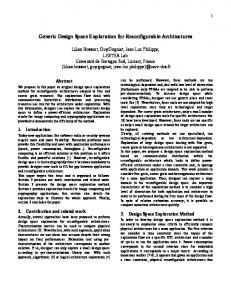
The principles mentioned above were a bit illustrated on the example of a conveyor named IUP (Berruet, Coudert, Kindler, 2004), but then now possibilities were discovered. While in the first illustration the internal anticipation concerned only the question whether the transitic system with failed working area(s) will be able to supply its normal function (and how long it will be able to do so), nowadays the anticipation concerns the question of the future operation when some components of the system have failed and according it the system is reconfigured. Let us explain it in more details. The description of the physical architecture can be seen in Fig. 1. It consists of a great cycle called main ring and of five working areas (WA1 to WA5). Parcels enter the main ring at the beginning of its lower long component and are transported to working places according with their technological programs. The transport proceeds according with the arrows. Both the long components of the main ring carry the parcels by motorized rollers while all other components of the system are deserved by pneumatic jacks. Parcels can be stopped due to mechanical stops. At a working area, a parcel can access subsequently three places α, β and γ. The parcel is manufactured at β, but it can enter a working area and wait at its place α, if β is occupied. When a parcel has been manufactured it comes to place γ and then can leave the working area for the main ring. In case its injection on the main ring could cause a crash with another parcel there, it has to wait at γ. The elaborated parcels leave the conveyor at the same place where they entered. In the presented example, every working area can implement two different transformation functions. WA1 and WA5 can perform F1 and F2, WA2 and WA3 can perform F2 and F3, and WA4 can perform F1 and F3. WA5 WA5
WA4 WA4
WA3 WA3
I/O WA1 WA1
WA2 WA2
Fig. 1: Static structure of the conveyor IUP
The logical description of the application is mainly performed by the introduction of the concept of Logical Operating Sequence (Log.Op.Seq.). A Log.Op.Seq. is a set of ordered machining functions applied to a family of parts. A function describes a service which the system (FMS) can deliver without allocated resource. Two Log.Op.Seq – (F1,F2,F3) and (F3,F2,F1) are considered in our example. The adopted configuration system architecture is the following. All the workshop is in normal operating mode (no element is in failure). WA1, WA2 and WA4 are in production (exploitation) mode (they are used for the current production), WA3 is put on standby mode (under tension, but not solicited), WA5 is not under tension (stop mode). 4.2
Tool description
A computer modeling tool has been developed. By parametrizing and other manipulation, having use mainly of the oject-oriented development of its generic headstones, the tool can be used as the model figuring in the definition of the anticipation systems by Rosen. It is based on the use of components that provide an easy way to build the different models and the internal one, too. Different rules govern the parcels movements. These rules are changed according with a structural change at the level of the system, a conclusion expressed by an internal simulation. Different experiments were carried out. As it was already mentioned by Berruet, Coudert and Kindler (2004), the first experiments applied a simulation model M of a rather simple system, in which there was no difference among the coming parcels: each of them was supposed to expect one processing step that was possible to be performed at any of the five existing working areas. During the run of M, the operator could model a failure occurrence, signaling a change of state of the corresponding working area WAi, where i is the hit key. The model M reflected the fact that the computer controlling the system simulates possible consequences of the change of state of WAi and displays them by animation. Next development consisted in adding rules for the processing of the parcels. Referring to the example above, the parcels were classified into two sorts so that each of the sorts had its proper Logical Operating Sequence. Each Log.Op.Seq. is composed of three machining functions. For any Log.Op.Seq., working areas were defined that should be able to perform it. In the following step of the development, the initial input of data allowed the operator to introduce statistical laws for the duration of the processing at any working area. At the disposal of the operator, normal, exponential and uniform distribution models exist, and a deterministic one (i.e. constant) as well. Similar choice is offered for the time intervals between parcels entering the system. That allows simulating cases when the functions are originally affected to a certain working area with a short mean value of processing. After this area becomes no more accessible, the processing is switched to another working area having its mean value of processing notably greater. That practice enables a large spectrum of simulation experiments. Fig. 2 displays a reflective simulation of the system Fig. 1. The animation of the external model is at the lower part of the display while the animation of the internal model takes place at the upper part. When the external model runs WA3 and WA5 are not used according with the initial configuration. When a failure affecting WA1 is considered, the internal model is
projected at the upper part of the display simulating one other system configuration (the case of the activation of WA3), while the lower part of the display is frozen. In the same figure, one can see that the external model called the internal one at time 878.5973. This internal model now shows what could happen at time 1398.0351 using another configuration where WA1 is out of order, WA2, WA3, WA4 are set in production mode. Near the time information, one can see the images of the queues of the parcels that are waiting to be accepted to the conveyor (one can see that the queue concerning the internal model has a bit grown). This enables to compare the future of the current configuration where WA1 is out of order with another possible configuration. For taking the snapshot the internal model run had to be interrupted. That was performed by an abrupt change of the continuous regime into the step-by-step one. The used software allows doing it from the keyboard. In the step-by-step regime, the simulated time of the running model appears at the bottom of the crane window. One can see there the value 1398.0351, too.
WA5
WA4
WA1
WA5
WA3
WA2
WA4
WA1
WA3
WA2
Fig. 2: Reflective simulation of IUP conveyor
Every parcel situated on the conveyor is mapped as a field containing a sequence of three symbols (for example, at WA4 of the external model we can watch two fields 3A1 and 3B1). The first symbol identifies the operational sequence, the second symbol represents the order of expected operation and the last symbol informs on the number of cycles that the parcel has performed over the main ring. The instantaneous states of the parcels are represented also by colors of the fields. The symbols XXX say the corresponding WA to be out of order. 5 CONTRIBUTION OF REFLECTIVE SIMULATION FOR RECONFIGURABLE SYSTEMS Based on the tool presented in section 4.2, experiments emphasized the interest of reflective simulation in case of anticipation of anticipating reconfigurable systems. At the beginning, the configuration of the system is simulated in its initial configuration. Its external model is computed. At a time t, a perturbation is introduced. It can be a failure occurrence or unexpected manufacturing order. The current configuration is no more suitable. Different configurations are then generated. For each of them, it is possible to simulate the system behavior and to calculate some parameters such as the number of manufactured parts and the mean waiting time. After, it is possible to return to the external model with the selected configuration and to simulate its evolution until a new change occurs. For example, internal simulation shows that in the case of a failure affecting WA1, at the moment it occurs, it is suitable to switch to the new configuration: WA2, WA3 and WA4 are in production (exploitation) mode, WA1 is put on shut down mode, WA5 stay in stop mode. This configuration is sufficient according to the simulated processing times. There is no need setting WA5 in production mode. According with criteria expressed in (Berruet, et al., 2000), only significant reconfiguration is sufficient. The anticipation of possible consequences of the decisions and choice among the variants can be got by means of forward-looking simulation. The computer C that controls a given system S can be used to generate the decisions that are physically possible and then to simulate the future of S according with the generated decision. So reflective simulation enables to measure how C can come to a quite good decision. The interest is not only to simulate a system that can change its configuration according with its possibilities and production criteria, but also to simulate how the reconfiguration process based on simulation is suitable. The next part opens the discussion and presents some examples of questions, the answers of which are given by mean of reflective simulation. Questions can be classified at two different levels. The first level mainly concerns production objectives and performance evaluation. It can not be answer by mean of "classical" (not reflective) simulation if the internal simulation could not be omitted from the real system, as it could not be replaced by any other methods. Q1) A failure occurs at WAi that can be supplied by other working areas. The repair would cause an interruption of the whole system. The question is about the length of the queue of the parcels requesting the system. Simulation of the conveyor operating with four working areas can answer and therefore help in the decision whether the failure should be repaired immediately or after a series of parcels have been performed. Q2) Only four working areas belonging to a set W are used. The fifth area Q is currently stopped due to the maintenance of a processing element. A fault occurs to a working area P
belonging to W. The question is how long the conveyor will be able to work in a good manner in case Q supplies P. The second level concerns the interest of reconfigurable system and relevancy of the reconfiguration process. Q3) What should be the maximum size for reflective simulation? Does the evaluation of one configuration spend a lot of time? Do only two or three configurations should be evaluated? Q4) Is it interesting to add a lot of redundancies to the design system? As it is well known, redundancy has a cost. Reflective simulation of such a system can help designers in their choices by providing data from dependability point of view. Other questions concern the reconfiguration process itself. Q5) What is the interest of the reconfiguration from dependability point of view? Q6) Does this process be relevant in a transitional phase? The system with and without reconfiguration can be simulated and the impact of dependability aspects studied. 6 CONCLUSION After defining the notion of nested simulation, this work points out some applications of reflective simulation. The area of interest concerns reconfigurable manufacturing systems and particularly a decisional reconfiguration process based on predictive simulation. The advantage of the presented techniques is that it can be applied during the design phase of the system. It opens some interesting ways for the evaluation using simulation of this kind of process. Technically, another benefit is that the building of the internal model is automatically performed when needed and the current statement of the external model is transmitted for internal simulation. The tools have now to be exploited in details. Different experiments are to be carried out considering the both variation of parameters of system physical architecture (as machining speed, number of redundancies, …) and parameters of reconfiguration (time to react, to reduce the system stop for withdrawal, to minimize the tardiness in completing the process, …). The objective of the anticipation shall be to have a productive system with good performances on a wide time horizon including some failures. The reactive piloting problematic could then be tackled by these kinds of techniques. Reflective simulation is also able to anticipate whether the decision algorithms are able to be calculated during the evolution of the real system. The rate of the simulating computer can be introduced as a parameter for the reflective simulation. The presented software tool enables to integrate the internal simulation model as on of the dynamic systems existing in time together with the other elements of the system mapped in the external model. The nested simulation of the conveyors illustrated the abundance of stimuli that come from technology to anticipatory systems and plenitude of ways how to solve the related obstacles. Currently further works are: • to use scripts to automatically generate simulation experiments with different failure occurrences.
• to introduce some rules based on simulation to anticipate where is the most opportune WA to perform the next step of a logical operating sequence. This will induce another level of internal model. The reflective simulation will have depth two (depth one for the evaluation of the reconfiguration process with another level for the simulating computer that enables to choose the best working area). ACKNOWLEDGEMENT This work was supported by the Institutional research scheme MSM6198898701 of the Czech Ministry of Education, Youth and Sport. REFERENCES Berruet, P., Coudert, T., Kindler, E. (2004). Conveyors With Rollers as Anticipatory Systems: Their Simulation Models. In: D. M. Dubois (editor): Computing Anticipatory Systems CASYS 2003 – Sixth International Conference, Liege, Belgium, 11-16 August 2003. American Institute of Physics, Melville, New York [AIP Conference Proceedings Volume 718], pp. 582-592 Berruet, P., Toguyéni, A. K. A., El Khattabi, S., and Craye E. (2000). Toward an Implementation of Recovery Procedures for FMS Supervision. Computers in Industry, Vol. 43, 227-236 Brennan R., Fletcher M., Zhang X., Norrie D., “Reconfiguraton of Real-time Distributed Control Systems : An IEC 61499 Based Approach“, Proc. International Conference on Industrial Engineering and Product Management, Laval, 2001. Henry, S. , Zamai, E., Jacomino, M., “Real time reconfiguration of manufacturing systems”, Proc. IEEE SMC 2004, The Hague, pp. 4266-4271, October 2004. Kamach, O., L. Pietrac, E. Niel, “Multi-model approach for discrete event systems : application to operating mode management”, Proc. IEEE-IMACS CESA 2003, Lille, July 2003. Kindler, E. (2000a). Nesting Simulation of a Container Terminal Operating With its own Simulation Model. JORBEL (Belgian Journal of Operations Research, Statistics and Computer Sciences) 40, No. 3-4, 169-181. Kindler, E. (2000b). Chance for Simula. ASU Newsletter, 26, No. 1 (May), 2-26. Kindler, E. (2001). Computer Models of Systems Containing Simulating Elements. In: Daniel M. Dubois (editor): Computing Anticipatory Systems CASYS 2000 - Fourth International Conference, Ličge, Belgium, 7-12 August 2000. AIP (American Institute of Physics), Melville, New York, 2001 [AIP Conference Proceedings Vol. 573], pp. 390-399 K. Ruy, Y. Son, M. Jung., “Modeling and specifications of dynamic agents in fractal manufacturing systems”, Computers in Industry, vol. 52, pp. 161-182, 2003. Shen, W., Norrie, D.H., "Agent-based systems for intelligent manufacturing: a state of the art survey", Knowledge and information systems, Vol. 1, no. 2, pp. 129-156, 1999. SIMULA Standard (1986). SIMULA a.s., Oslo, 1986 Tomizuka, M (2002). Mechatronics: from the 20th to 21st century. In: Control Engineering Practice, 10, no 8, 877-886.