Networks that Learn for Image Understanding - Semantic Scholar

Networks that Learn for Image Understanding Tomaso Poggio and Kah-Kay Sung

Abstract Learning is becoming a central problem in trying to understand intelligence and in trying to develop intelligent machines. This paper describes some recent work on developing machines that learn in the domains of vision and graphics. We will introduce an underlying theory which connects function approximation techniques, neural network architectures and statistical methods. While these techniques have limitations, one can overcome these limitations by using the idea of virtual examples. We shall describe some learning-based systems we have developed that recognize objects, in particular faces, nd speci c objects in cluttered scenes, and produce novel images under user control. Finally, we will discuss about the implications of this research on how the brain might work. 1

1 Introduction Learning and vision are two very broad elds of research. In this paper we will introduce an underlying theory which connects supervised learning, function approximation techniques, neural network architectures and statistical methods. We shall make a few general observations about supervised learning approaches in vision. Then we will brie y describe some learning-based image understanding (IU) applications developed at the MIT Center of Biological and Computational Learning. Finally, we will discuss about the implications of this research on how the brain might work. Vision systems that learn and adapt represent one of the most important future directions in IU research. This re ects an overall trend { to make intelligent systems that do not need to be fully and painfully programmed. It may be the only way to develop vision systems that are robust and easy to use in many dierent tasks. Building systems without explicit programming is not a new idea. Duda and Hart [10] is still one of the best textbooks. However, there are extensions of the classical pattern recognition techniques, extensions often called Neural Networks. Neural Networks have provided a new metaphor { learning from examples { that makes statistical techniques more attractive. As a consequence of this new interest in learning, we are witnessing a renaissance of statistics and function approximation techniques and their applications to new domains such as vision.

1 This paper describes research done within the MIT Center for Biological and Computational Learning in the Department of Brain and Cognitive Sciences, and at the MIT Arti cial Intelligence Laboratory. This research is sponsored by grants from the Oce of Naval Research under contracts N00014-91-J-1270 and N00014-92-J-1879; by a grant from the National Science Foundation under contract ASC-9217041 (funds provided by this award include funds from DARPA provided under the HPCC program). Additional support is provided by the North Atlantic Treaty Organization, ATR Audio and Visual Perception Research Laboratories, Kodak, Daimler Benz and Siemens AG. Tomaso Poggio is supported by the Uncas and Ellen Whitaker Chair. Kah-Kay Sung is currently a lecturer at the Department of Information Systems and Computer Science, National University of Singapore.

xd)

xj,

x = (x1,

x1

xi

G

xN

G ci

c1

G cN

+

f(x)

(a)

(b)

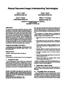
Figure 1. (a): Learning-from-examples as multivariate function approximation or interpolation from sparse data. Generalization means estimating f  (x)  f (x) ; 8x 2 X from the examples f (xi ) = f (xi), i = 1; : : :; N . (b): A Regularization Network. The input vector x is d-dimensional, there are N hidden units, one for each example xi, and the output is a scalar function f (x).

2 Learning-from-Examples as Multivariate Function Approximation

In this section we will concentrate on one aspect of learning: supervised learning. Supervised learning, or learning-from-examples, refers to systems that are trained, instead of programmed { by a set of examples, that is input-output pairs (xi ; yi). At run-time these systems would hopefully provide a correct output for a new input not contained in the training set. One can formulate supervised learning as a regression problem of approximating a multivariate function from sparse data, i.e. the examples (Figure 1(a)). Generalization means estimating the value of the function for points in the input space where data is not available. Once the ill-posed problem of learning-from-examples has been formulated as a function approximation problem, an obvious approach to solving it is regularization. Regularization imposes a constraint of smoothness on the space of approximating functions by minimizing the cost functional:

H [f ] = PNi=1 (yi ? f (xi ))2 + [f ];

(1)

where the stabilizer  is typically a measure of smoothness of the solution f . The functional regularization approach can also be regarded from a slightly more general probabilistic and Bayesian perspective. In particular, as Girosi, Jones and Poggio [15] [14] (see also Poggio and Girosi [23],[22] and Wahba [28]) describe, a Bayesian approach leads to the maximum a posteriori (MAP) estimate of P (f jD) / P (f ) P (Djf ) , where the set D = (xi; yi)Ni=1 consists of the input-output pairs of training examples. I the noise model is additive and Gaussian (i.e. P (Djf ) is Gaussian) and the prior P (f ) is a Gaussian distribution of a linear functional of f , then the MAP estimate, that is the f maximizing P (f jD), is equivalent to the f that minimizes equation (1).

2.1 Regularization Networks A key result is that under rather general conditions, the solution of the regularization cost functional in equation(1) can be expressed as a linear combination of basis functions (G), centered on the data points xi:

(2) f (x) = PNi=1 ci G(x ? xi) + p(x); The form of the basis function G depends on the smoothness prior, that is the functional . R 2 Speci cally, [f ] = jfG~~((ss))j ds, the operator ~ indicates the Fourier transform, and p(x) is a polynomial term that is not needed for positive de nite G such as the Gaussian function.

The solution provided by equation (2) can always be rewritten as a network with one hidden layer containing as many units as examples in the training set (see Figure 1(b)) [23] [8]. We call these networks Regularization Networks (RN). The coecients ci that represent the \weights" of the connections to the output are \learned" by minimizing the functional H over the training set.

2.2 Radial Basis Functions An interesting special case arises for radial . In this case the basis functions are radial and the network is

f (x) = PNi=1 ciG(kx ? xi k) + p(x):

Legal G's include the Gaussian, the multiquadric, thin-plate splines and others [22]. In the Gaussian case, these RBF networks consist of units, G(kx ? xik), each tuned to one of the examples, xi, with a bell-shaped activation curve. The examples, xi , which are the unit centers, behave like templates. \Vanilla" RBFs can be generalized to the case in which there are fewer units than data, and the centers xi are to be found during the learning phase of minimizing the cost over the training set. A weighted norm can also be introduced instead of the Euclidean norm and again the associated matrix can be found during the learning phase. These generalized RBF networks have sometimes been called HyperBF networks [22].

3 Three observations Given this general framework for looking at the problem of learning-from-examples, three observations are relevant.

3.1 Regularization Provides a General Theory The rst point is summarized in Figure 2: several representations for function approximation and regression as well as several Neural Network architectures can all be derived from regularization principles with somewhat dierent prior assumptions on the smoothness of the function space (the stabilizer ). They are therefore quite similar to each other. In particular, the radial class of stabilizer is at the root of the techniques on the left branch of the diagram: RBF can be generalized into HyperBF and into some kernel methods and various types of multidimensional splines. A class of priors combining smoothness and additivity [15] is at the root of the middle branch of the diagram: additive splines of

many dierent forms generalize into ridge regression techniques, such as the representations used in Projection Pursuit Regression [12], hinges [7] and several multilayer perceptron-like networks (with one hidden layer).

3.2 The Learning-from-Examples Framework almost implies a View-based Approach to Object Recognition The second general point is that the simplest version of an example-based approach to object recognition { and, as we will see later, to graphics { is equivalent to a view-based approach to recognition. Consider a learning-from-examples network trained to classify dierent views of a 3D object against views of other distractor objects. Suppose the network has a Gaussian Radial Basis Function form. Then, as discussed by Logothetis, et al. [19] [20], each hidden unit is view-tuned to one of the example views, whereas the output can be view invariant but object speci c (if a sucient number of examples and units are available).

3.3 Prior Information is needed to Leverage the Example Set The third and last observation has to do with sample complexity { how many \training examples" are needed for a supervised learning scheme to reasonably solve a speci c problem. Niyogi and Girosi [18] have recently proven the following result, which extends to Radial Basis Functions results due to Barron [2] for multilayer perceptrons:

Theorem 1 Let f 2 H m; (Rd), where H m; (Rd) is the space of functions whose partial 1

1

derivatives up to order m are integrable, and let m > d, with m even. Let fn;N be a Gaussian basis function network, with n coecients, n centers and n variances, that has been trained on a set of N data points. Then, with probability 1 ?  , the generalization error is bounded by the following inequality:

1

.

E [(f ? fn;N )2 ] < O n

0  12 1 nd ln( nN ) ? ln  A +O@ N

The plot of Figure 3 summarizes the main result of the theorem. Generalization error on new data, not used for training, depends on the number of examples N and on the complexity of the network, described here by the number of its free parameters n. Notice that for each N there is an optimal n. In many cases, especially when N is not very large, the choice of a good n is often more important in practice than the choice of one regression or classi cation architecture vs. another. The main point here is however a simpler one: very often we are forced to work in the region of the plot with very small N , i.e., there is not enough training data. This, we believe, is one of the most basic limitations of all the nonparametric learning-from-examples schemes. What can be done? Poggio and Vetter [24] have pursued the idea of exploiting prior information about the speci c problem at hand to generate virtual examples and thus expand the size of the training set, that is N . We shall describe speci c instances of this approach for face recognition and face detection.

Regularization networks (RN) Generalized Regularization Networks (GRN)

Regularization Radial Stabilizer

Additive Stabilizer

Additive Splines

RBF

Movable metric Movable centers

Movable metric Movable centers

HyperBF if ||x|| = 1

Product Stabilizer

Tensor Product Splines

Movable metric Movable centers

Ridge Approximation

Figure 2. Several classes of approximation schemes and corresponding network architectures can be derived from regularization with the appropriate choice of smoothness priors, associated stabilizers and basis functions. From Girosi, Jones, and Poggio (1995).

Figure 3. An

illustration of the theorem. From Niyogi and Girosi (1994).

4 Learning-from-Examples for Image Understanding We now describe three speci c projects in our group that use the learning-from-examples techniques for approaching problems in computer vision and computer graphics, using human faces as the class of 3D objects.

4.1 Example-based Image Analysis and Image Synthesis In the image analysis problem, a learning module is trained to associate input images to output parameters { such as the classi cation label for the object in the image and possibly pose and expression parameters associated with it. After training with a set of images and corresponding parameters, the network is expected to generalize correctly; that is, to classify new views of the same object, recognize another object of the same class, or estimate its pose/expression parameters. In the \inverse" problem of image synthesis, a learning module is used to associate input parameters to output images. This module synthesizes new images and represents a rather unconventional approach to computer graphics. It takes several real images of a possibly non-rigid 3D object, and creates new images by generalizing from those views, under the control of appropriate pose/expression parameters assigned by the user during the training phase.

4.1.1 The Analysis Network

Given a set of example images labeled in pose and expression space (see Figure 4(a)), a RBF network (see equation (2)) can be trained to estimate the pose-expression parameters of new images of the same person. The network input, or our image representation, is a geometrical representation of (x; y ) locations of facial features as pixel-wise correspondence with respect to a reference image [3], here chosen to be the upper left image in Figure 4(a). There are two parameters in the output, representing the amount of smile and rotation of the face. The network is constructed using four Gaussian RBF hidden units, one for each of the example images. After \training" with the four examples the network can \generalize" to new images of the same person, estimating the associated rotation and smile parameters. Examples of input images and their estimated parameters are shown in Figure 5(b).

4.1.2 The Synthesis Network

In the synthesis case the role of inputs and outputs are exchanged. Figure 5(a) shows the network [3] used to synthesize images of a speci c person's face under control of two poseexpression parameters, the same ones used by the analysis network. For network output, since our image representation uses pixel-wise correspondence with respect to a reference image, the number of outputs, q , is twice the number of pixels in the image (each pixel has an x and y coordinate). The output geometry produced by the network is then \rendered" by applying 2D warping operations to the example image \textures". Figure 4(b) shows some example images generated by the synthesis network. The four examples used here are the same as for the analysis case and are shown at the four corners of the gure. All the other images are \generalizations" produced by the network after the \learning" phase.

0

-x

1 x

0 img 1

img 2

img 3

img 4

1

y

?

y

(a)

(b)

(a): In our demonstrations of the example-based approach to image analysis and synthesis, the example images img1 through img4 are placed in a 2D rotation-expression parameter space (x; y ), here at the corners of the unit square. For analysis, the network learns the mapping from images (inputs) to parameter space (output). For synthesis, we synthesize a network that learns the inverse mapping, that is the mapping from the parameter space to images. From Beymer et al. (1993). (b): Multidimensional image synthesis using the example images bordered in black. All other images are generated by the synthesis network. From Beymer et al. (1993) .

Figure 4.

X

1

...

X

d

) ...

G1

+

+

y1

...

y2 . . .

...

+

...

...

GN

+ yq − 1

(a)

(x; y ) = (0:958; 0:056) + yq

) (x; y ) = (0:152; 0:810)

(b)

(a): The network used to synthesize images from pose inputs. It diers from the Regularization Network in Figure 1(b) simply by having more outputs, q in this case. Since we use a pixel wise representation for our output images, q is proportional to the number of pixels in the image. (b): In each of the boxed image pairs, the novel input image on the left is fed into an analysis RBF network to estimate rotation x and expression y . These parameters are then fed into the synthesis module of gure 4(b) that synthesizes the image shown on the right. This gure can be regarded as a very simple demonstration of very-low bandwidth teleconferencing: only two pose parameters need to be transmitted at run-time for each frame. From Beymer et al. (1993) .

Figure 5.

4.1.3 Very-low Bandwidth Video E-Mail

The analysis and the synthesis network can each be used independently for a variety of applications. A particularly interesting application is very-low bandwidth video e-mail and video-conferencing. Figure 5(b) shows a demonstration of the basic idea. An analysis network trained on a few views of the speci c user analyzes new images during the session in terms of a few pose and expression parameters. These few parameters are sent electronically for each frame and used at the receiver site by a similar synthesis network to reconstruct appropriate new views. This model-based approach can achieve in principle very high compression.

4.2 Face Recognition We will now summarize our work over the last 4 years on face recognition, rst covering two view-based face recognition systems that rely on several example views per person. We will then discuss work on synthesizing virtual example views to deal with situations where only one example view (also called model view) per person is available.

4.2.1 The Brunelli-Poggio frontal face recognition system

Following the face recognition work of Baron [1], Brunelli and Poggio [9] use a templatebased strategy to recognize frontal views of faces. From an example model view, faces are represented using templates of the eyes, nose, mouth, and entire face. A normalized correlation metric is used to compare the model templates against the input image. During recognition, input images are geometrically registered with the model views by aligning the eyes, which normalizes the input for the eects of translation, scale, and imageplane rotation. On a data base of 47 people, 4 views per person, the recognition performance is 100% when two views are used as model views and the remaining two views are used for testing. Using an algorithm very similar to the Brunelli-Poggio system, Gilbert and Yang [13] have also developed a fast PC-based face recognition system that uses custom VLSI chips for correlation.

4.2.2 The Beymer pose-invariant face recognition system

In a view-based extension of the Brunelli-Poggio system, Beymer [5] [6] developed a poseinvariant face recognizer that uses 15 views per person, views that cover dierent out-ofplane rotations (see Figure 6). As in the previous system, translation, scale, and imageplane rotation are factored out by rst detecting eyes and nose features and then using these features to register the input with model views. To recognize a new input, the image is matched against all model views of all people and the best match is reported. The matching step performs normalized correlation using eyes, nose, and mouth templates. On a data base of 62 people and 10 test views per person, the system obtained a recognition rate of 98%.

4.2.3 Face Recognition with Virtual Views

As discussed previously, the key problem for the practical use of learning-from-examples schemes { and for non-parametric techniques in general { is often the limited size of the training set. Recently, we have seen how one can exploit prior knowledge of symmetry properties in 3D objects to synthesize additional training examples [24]. The idea is to

Figure 6. The

pose-invariant, view-based face recognizer uses 15 views to model a person's face. From Beymer (1993) .

prototype

novel person (B)

(A) prototype flow

(a)

Figure 7.

(C) mapped prototype flow

virtual view

(b)

(a): In parallel deformation, (A) a 2D deformation representing a transformation

is measured by nding correspondence among prototype images. In this example, the transformation is rotation and optical ow was used to nd a dense set of correspondences. Next, in (B), the ow is mapped onto the novel face, and (C) the novel face is 2D warped to a \virtual" view. From Beymer and Poggio (1995b) . (b): A real view (center) surrounded by virtual views derived from it using parallel deformation. From Beymer and Poggio (1995b) .

learn class-speci c transformations from example objects, and synthesize virtual views of new objects in the same class from a single view. Figure 7(a) [4] shows one way of generating virtual face views by applying a transformation \learned" from prototypes of the same class (faces). Called parallel deformation [21], a 2D deformation measured on the prototype faces is mapped onto the novel face. The mapped deformation then drives a 2D warping of the novel face to the virtual view. Figure 7(b) shows the result of applying this technique to produce several rotated virtual views of the same face from a single real image. The virtual views generated in this way have been used as model views in the poseinvariant recognizer described earlier to achieve recognition rates that are likely to compare well to human performance in the same situation [4].

4.3 Example-based Face Detection Our last project deals with the general problem of object and pattern detection in cluttered pictures. It has been often said that this problem is even more dicult than the problem of isolated object recognition [16]. We have developed [27] [25] an example-based learning approach for locating vertical frontal views of human faces in cluttered scenes. The approach uses learning-based methods to complement human knowledge for capturing complex variations in face patterns.

4.3.1 Learning a Distribution-based Face Model

The rst learning task is to build a distribution-based model for describing possible variations in face image appearances (see Figure 8). We use a representative sample of face patterns to approximate the distribution of frontal face views in a normalized 19  19 pixel image vector space. We also use a carefully chosen sample of \face-like" non-face patterns to help localize the boundaries of the face distribution. The nal model consists of a few (6) elongated Gaussian \face" clusters that coarsely describe the frontal face pattern distribution in the 19  19 pixel image vector space, and a few (6) \non-face" clusters that explicitly carve out regions in the image vector space that do not correspond to face views. One can interpret these model clusters as a set of view-based \face" and \non-face" prototypes in a HyperBF object recognition network architecture.

4.3.2 Learning a Similarity Measure for Identifying Face Patterns

To search for faces at dierent image locations and scales, our system resizes each square image window to 19  19 pixels and matches the resized pattern against the distribution-based face model. The matching stage computes a \dierence" feature vector of 12 directionally dependent distances between the resized pattern and the 12 model centers. Here, we also use example-based learning techniques to train a network classi er that identi es face patterns from non-face windows, based on their \dierence" feature vector measurements with the model. For this stage, our experiments have shown that the choice of one network architecture vs. another is not very crucial.

4.3.3 Virtual Example Generation and Example Selection

Figures 9 and 10(a) show some face detection results by our system. For high quality CCD images, the system has a 96:3% face detection rate with an extremely low false alarm rate. The system's robust performance was largely due to the way we used virtual views to

Figure 8. Our distribution-based face model. Top Row: We use a representative sample of frontal face patterns to approximate the distribution of frontal face views in a normalized 19  19 pixel image window vector space. We model the face sample distribution with 6 multi-dimensional Gaussian clusters whose centers are as shown on the right. Bottom Row: We use a carefully chosen sample of non-face patterns to help localize the boundaries of the face distribution. We also model the non-face sample distribution with 6 multidimensional Gaussian clusters. The nal model consists of 6 Gaussian \face" clusters and 6 \non-face" clusters.

signi cantly increase the number of face training patterns. We generated 3000 virtual face examples by applying some simple image transformations to the 1000 real face views we had in our training database. For practical reasons, we also had to constrain the number of non-face patterns in our training data set without unnecessarily sacri cing the quality of negative examples. To do this, we used an incremental scheme for selecting high quality non-face training examples [25] [26]. The scheme starts with a small number of non-face patterns in the training database, and gradually adds new non-face patterns that the current system wrongly classi es as faces.

5 Object Recognition | Psychophysical and Physiological Connections As shown in the previous sections, the example-based approach is successful in practical problems of object recognition, object detection, image analysis and image synthesis. We conclude by asking whether a similar approach may be used by the human brain. Over the last four years, psychophysical experiments have indeed supported the example-based

Figure 9. Some

face detection results. From Sung and Poggio (1994) .

X1

•

•

•

•

•

Xd

•

+

(a)

(b)

(a): More face detection results. The same system nds real faces as well as hand drawn faces. From Sung and Poggio (1994). (b): A RBF network with four units

Figure 10.

each tuned to one of the four training views shown in the next gure. The tuning curve of each of the unit is also shown in the next gure. The units are view-dependent and selective, relative to distractor objects of the same type.

HIDDEN UNITS

NETWORK x target ... distractors

Figure 11. Tuning of each of the four hidden units of the network of the previous gure for images of the \correct" 3D objects. The tuning is broad and selective: the dotted lines indicate the average response to 300 distractor objects of the same type. The bottom graphs show the tuning of the output of the network after learning (that is computation of the weights c): it is view-invariant and object speci c. Again the dotted curve indicates the average response of the network to the same 300 distractors. From Vetter and Poggio (unpublished).

and view-based schemes that we suggested as one of the mechanisms for object recognition. Very recently, physiological experiments have also provided a suggestive glimpse on how neurons in IT cortex may represent objects for recognition. The experimental results seem to agree surprisingly well with our model [17]. Figure 10(b) shows our basic module for object recognition. Classi cation or identi cation of a visual stimulus is accomplished by a network of units. Each unit is broadly tuned to a particular view of the object. We refer to this optimal view as the center of the unit. One can think of each unit center as a template to which the input is compared. The unit is maximally excited when the stimulus exactly matches its template but also responds proportionately less to similar stimuli. The weighted sum of activities of all the units represents the output of the network. Consider how the network \learns" to recognize views of the object shown in Figure 11. In this example the inputs of the network are the (x; y ) positions of the vertices of the wireframe object in the image. Four training views are used. After training, the network consists of four units, each one tuned to one of the four views as in Figure 11. The weights of the output connections are determined by minimizing misclassi cation errors on the four views and using as negative examples views of other similar objects (\distractors"). The graphs show the tuning of the four units for images of the \correct" object. The tuning is broad and centered on the the training views. Somewhat surprisingly, the tuning is also very selective: the dotted line shows the average response of each of the unit to 300 similar distractors [11]. Even the maximum response to the best distractor is in this case always less than the response to the optimal view. Despite its gross oversimpli cation, our model relates well to some recent psychophysical and physiological ndings, in particular to the existence of view-tuned and view-invariant neurons in the primate IT cortex, and to the shape of psychophysically measured recognition elds. We refer interested readers to the following pieces of work by Logothetis and coworkers for further details [17], [19] [20].

References [1] Robert J. Baron. Mechanisms of human facial recognition. International Journal of Man Machine Studies, 15:137{178, 1981. [2] A.R. Barron. Approximation and estimation bounds for arti cial neural networks. Machine Learning, 14:115{133, 1994. [3] D. Beymer, A. Shashua, and T. Poggio. Example based image analysis and synthesis. AIM-1431, AI Lab., MIT, 1993. [4] David Beymer and Tomaso Poggio. Face recognition from one example view. In Proceedings of the International Conference on Computer Vision, pages 500{507, Cambridge, MA, June 1995. [5] David J. Beymer. Face recognition under varying pose. AIM-1461, AI Lab., MIT, 1993. [6] David J. Beymer. Face recognition under varying pose. In Proceedings IEEE Conf. on Computer Vision and Pattern Recognition, pages 756{761, Seattle, WA, 1994. [7] L. Breiman. Hinging hyperplanes for regression, classi cation, and function approximation. IEEE Transaction on Information Theory, 39(3):999{1013, May 1993. [8] D.S. Broomhead and D. Lowe. Multivariable functional interpolation and adaptive networks. Complex Systems, 2:321{355, 1988.

[9] R. Brunelli and T. Poggio. Face recognition: Features versus templates. IEEE Transactions on Pattern Analysis and Machine Intelligence, 15(10):1042{1052, 1993. [10] R. O. Duda and P. E. Hart. Pattern Classi cation and Scene Analysis. Wiley, New York, 1973. [11] S. Edelman and H. H. Bultho. Orientation dependence in the recognition of familiar and novel views of 3D objects. Vision Research, 32:2385{2400, 1992. [12] J.H. Friedman and W. Stuetzle. Projection pursuit regression. Journal of the American Statistical Association, 76(376):817{823, 1981. [13] J.M. Gilbert and W. Yang. A real-time face recognition system using custom VLSI hardware. In IEEE Workshop on Computer Architectures for Machine Perception, pages 58{66, New Orleans, LA, December 1993. [14] F. Girosi, M. Jones, and T. Poggio. Priors, stabilizers and basis functions: From regularization to radial, tensor and additive splines. AIM-1430, AI Lab., MIT, 1993. [15] F. Girosi, M. Jones, and T. Poggio. Regularization theory and neural networks architectures. Neural Computation, 7:219{269, 1995. [16] A. Hurlbert and T. Poggio. Do computers need attention? Nature, 321:651{652, 1986. [17] N.K. Logothetis and J. Pauls. Psychophysiological and physiological evidence for viewer-centered object representations in the primate. Cerebral Cortex, 5:270{288, 1995. [18] P. Niyogi and F. Girosi. On the relationship between generalization error, hypothesis complexity, and sample complexity for radial basis functions. AIM-1467, AI Lab., MIT, 1994. [19] N.K. Logothetis, J. Pauls and T. Poggio. View-dependent object recognition by monkeys. Current Biology, 4:401{414, 1994. [20] N.K. Logothetis, J. Pauls and T. Poggio. Shape representation in the inferior temporal cortex of monkeys. Current Biology, 5:552{563, 1995. [21] T. Poggio and R. Brunelli. A novel approach to graphics. AIM-1354, AI Lab., MIT, 1992. [22] T. Poggio and F. Girosi. Networks for approximation and learning. Proceedings of the IEEE, 78(9), September 1990. [23] T. Poggio and F. Girosi. Regularization algorithms for learning that are equivalent to multilayer networks. Science, 247:978{982, 1990. [24] T. Poggio and T. Vetter. Recognition and structure from one 2D model view: observations on prototypes, object classes and symmetries. AIM-1347, AI Lab., MIT, 1992. [25] K. Sung. Learning and Example Selection for Object and Pattern Detection. PhD thesis, Massachusetts Institute of Technology, Cambridge, MA, 1995. [26] K. Sung and P. Niyogi. Active learning for function approximation. In Advances in Neural Information Processings Systems 7, pages 593{600, MIT Press, 1995. [27] K. Sung and T. Poggio. Example-based learning for view-based human face detection. In Proceedings from Image Understanding Workshop, Monterey, CA, 1994. [28] G. Wahba. Splines Models for Observational Data. Series in Applied Mathematics, Vol. 59, SIAM, Philadelphia, 1990.