1
Neural Network Automatic Test Pattern Generator Priyanka Sinha Department of Electrical and Computer Engineering, Auburn University 200 Broun Hall, AL-36849
[email protected]
Abstract— This paper discusses the technique for modeling a test generation problem using neural networks. Through examples, it illustrates the representation of a digital circuit as a hopfield network; the translation of faults to the same and the generation of test vectors for it. The results that have been reported, clearly indicate the advantage in using it as a means of parallelizing the test generation process.Further, faster ways of implementing the energy minimization using quadratic 0-1 programming are discussed.
•
AND Tij Ii K
•
Tij
Vi
•
Ii
(1 − δ (i, j)) × ((A + B) × connected (i, j) − B × inputs (i, j)) = −B × output (i) − A × input (i)
K
=
Ii K
= 0 if ΣN j=1 Tij Vj > 0 = Vi otherwise
Ii K •
0
=
(1 − δ (i, j)) ×
((−A − B) × connected (i, j) − B × inputs (i, j)) = −B × output (i) − A × input (i) = 0
NOR Tij
= 1 if ΣN j=1 Tij Vj < 0
=
NAND Tij
•
(1 − δ (i, j)) ×
((A + B) × connected (i, j) − B × inputs (i, j)) = − (2A + B) × output (i) = 0
OR
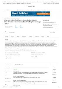
I. I NTRODUCTION Automatic test pattern generation for a large combinational circuits testing is frequent for VLSI circuits. Therefore, parallelizing the process would helps in reducing the time for testing. In order to truly do so, the testing problem has to be mapped to a parallel computation model. Neural networks are useful represent complex non-linear functions. A hopfield network is a kind of neural network that has been used here. They are an attempt to model the vastly parallel collection of neurons in our brain. The neurons are depicted as a set of nodes related by bidirectional weighted edges of weight T ij. Each node has an activation state V associated with it and a threshold I. The network is in an excited state if upon randomly updating a neuron, according to the update rule given as
=
=
(1 − δ (i, j)) × ((−A − B) × connected (i, j) − B × inputs (i, j))
= B = B
NOT Tij
, its state changes depending on the state of its neighbours. Where N is the number of nodes in the network and the energy E is given by 1 ΣN Tij V iV j − ΣN E = − ΣN i=1 IiV i + K 2 i=1 j=1 , K being a constant. If the state does not change with the update rule, then the network is in stable state. Hopfield has proved that in the stable state the energy is the minimum. Hence, such a neural network can be used to model an optimization problem by defining the energy function appropriately and allowing the network to stabilize by randomly updating the nodes. This is the inherent parallelization in the model. The weights of the hopfield network are determined by the training vector sequences that are fed to the network, which in the case of AND,OR,NOT,NAND and NOR gate are simple functions given by
= −2J × (1 − δ (i, j))
Ii K
= − (2A + B) × output (i) = 0
where the functions are as follows: inputs (i, j)
connected (i, j) δ (i, j) output (i) input (i)
=
1 if i and j are input neurons f or the same gate
0 otherwise = 1 − inputs (i, j) = 1 if i = j =
0 otherwise 1 if i is an output neuron f or the gate
0 otherwise = 1 if i is an input neuron f or the same gate 0 otherwise
2
This idea of representation to be used for an ATPG is defined by [1]. Section I presents the history of the idea of neural networks being used for automatic test pattern generation. Section II illustrates an example of how a neural network can be used to generate tests. Section III depicts the and Section IV concludes.
are merged in the step of neural pruning. Then, the energy minimization would generate a test for the faulty circuit. After all of this, the optimizations are made to expend minimum effort in generating the test. In the following sections we go over these steps taking the example circuit to be Figure 2, i.e., a = N OT (b) c = AN D(a, b)
II. BACKGROUND Neural networks have been an object of study since the 1940’s. The Hopfield network has been around since 1982. Its uniqueness is in the fact that it is a recurrent network, i.e., it has feedback loops from the output to its input which gathers the associative nature of the neurons in the brain closer than back propagation . Hopfield had solved the problem of defining a recurrent neural network that would surely stabilize. By 1985, it was known that these Hopfield networks could be used to solve combinatorial optimization problems. The challenge lay in modelling such a problem in terms of a Hopfield network.Figure ??
d
Fig. 2.
Fig. 1.
A hopfield network
In the area of testing, in the attempt to reduce the time to test massive circuits, which VLSI would end up with, a major effort would be underway to parallelize the test generation problem in order to reduce that time. The technical report, ”Automatic Test Generation using Neural Networks” , 1988’ is the earliest I could find that had a mention of using neural networks for test generation. The following publications [?], [2], [3], [8] are compiled into the book [1]. The initial use of a gradient descent technique to minimize the energy function cleared the validity of the model for stuck-at faults. Later on, the minimization was made faster using the idea of implication graphs. Transitive closure and path sensitization could detect redundant faults and also model delay tests. The latest point of interest is in [?] and [11]. Further interest in the implication graphs were presented by VD Agrawal.
= OR(a, c)
Example Circuit
This circuit has a total of 16 stuck at faults of which m-s-a-0 and c-s-a-0 are redundant and (b-s-a-0, a-s-a-1, l-s-a-1, m-s-a-1, c-s-a-1, d-s-a-1) and (b-s-a-1, a-s-a-0, l-s-a-0, d-s-a-0) are equivalent. States NoFault b-s-a-0 b-s-a-1 a-s-a-0 a-s-a-1 l-s-a-0 l-s-a-1 m-s-a-0 m-s-a-1 c-s-a-0 c-s-a-1 d-s-a-0 d-s-a-1 b=0 1 1 0 0 1 0 1 1 1 1 1 0 1 b=1 0 1 0 0 1 0 1 0 1 0 1 0 1
A. Represent a digital circuit as a neural network Using the functions for thresholds and activation values given above, and taking the circuit Figure 2 as a sample circuit, the weights and thresholds have been calculated and shown in 3. IV. R EPRESENT A FAULT IN A CIRCUIT
III. A NALYSIS AND A LGORITHMS In order to use neural networks for test generation, the circuit under test has to be represented as a neural network. After this novel step, the fault in the circuit is modeled. If possible, nodes with equal threshold, inputs and output
Using the same circuit, the fault l-s-a-1 is represented as Figure 4. For the faulty node, a dual node a“ is created. All nodes related to ’a” as output of the AND gate are connected to its non-fault node ’a’. All nodes related to ’a’ as input are connected to its faulty node ’a“’. This results in Figure 5 is the
3
Where, E k for each of the nodes is given by Ek
= E (Vk = 0) − E (Vk = 1) = Ik + ΣN j=1 Tjk Vj
Now, to generate a valid assignment for the Figure 2, we start initially with 0 activation value for each of the neurons, which leads to energy of 2.
Va = 0 Vb = 0 Vc = 0 Fig. 3.
Vd = 0
Example Circuit converted to a Hopfield Network
network for both the good and faulty values. The activation value for a”’, Va”’ is held at 1 and for a’ and a at 0 to represent fautl sensitization and stuck-at-1 fault.
ECKT
= EN OT (Va Vb ) + EAN D (Va Vb Vc )
EAN D
+EOR (Va Vb Vc ) = −1/2(Tab Va Vb + Tbc Vc Vb + Tca Va Vc ) −(Ia Va + Ib Vb + Ic Vc ) + K
EOR
= −1/2(Tad Va Vd + Tdc Vc Vd + Tca Va Vc ) −(Ia Va + Id Vd + Ic Vc ) + K
EN OT
= −1/2(Tab Va Vb + Tab Vb Va ) −(Ia Va + Ib Vb ) + K
ECKT
=0
Then, we randomly perturb, this or that neuron and find out that updating b changes its state to 1, which gives the energy for the circuit to be -2 which is less than 0 and hence we obtain the consistent assignment as V a=0,V b=1,V c=0,V d=0. This is known as the gradient descent technique with iterative relaxation. Using the same procedure, the consistent assignment is obtained for the neural network described for the faulty circuit Figure 5. VI. R ESULTS Fig. 4.
Example Circuit with l-s-a-1 fault
V. T EST GENERATION In order to generate a test, the energy of the system has to be minimized which will happen in the case of stable state. The energy of the circuit is formulated as : ECKT
= EN OT (Va , Vb ) + EAN D (Va , Vb , Vc ) + EOR (Va , Vc , Vd )
The update rule for every random perturbation of the nodes is given by Vk
=
1 if Ek > 0 0 if Ek < 0 Vk otherwise
The results reported by [1] clearly indicate the advantage in using this model for test generation and it being an effective way to parallelize the circuit. They show that less than 1 sec is taken to test the either the Schneider Circuit, the 4-bit parallel adder(SN5483A) or the ECAT. No fault simulator was used and the number of tests are less than the number of tests,i.e., test vectors are compact to a certain degree. Figure 6 VII. C ONCLUSIONS Thus, this technique is definitely valid and workable for test generation. It gives rise to not only a solution to testing but has implications on various other fields as well. R EFERENCES [1] Neural Models and Algorithms for Digital Testing, Srimat T Chakradhar, Vishwani D. Agrawal, Michael L. Bushnell, Kluwer Academic Publishers. [2] Automatic Test Generation Using Neural Networks , Srimat T Chakradhar, Michael L. Bushnell, Vishwani D. Agrawal,
4
[3] Toward Massively Parallel Automatic Test Generation, SRIMAT T. CHAKRADHAR, MICHAEL L. BUSHNELL, VISHWANI D. AGRAWAL [4] NEUDEM Neural network based decision making for generating tests in digital circuits. Suresh Rai, H. Lee Johnson, and Vijay Ratnam. [5] Generalized Hopfield Neural Network for Concurrent Testing, Julio Ortega, Alberto Prieto, Antonio Lloris, and Francisco J. Pelayo [6] Neural Networks As Massively Parallel Automatic Test Pattern Generators, A. Majumder, R. Dandapani [7] Neural Models for Transistor and Mixed-Level Test Generation, Carolina L. C. Cooper, Michael L. Bushnell [8] Redundancy Identification Using Transitive Closure. Vishwani D. Agrawal, Michael L. Bushnell, Qing Lin [9] COGENT: Compressing and compacting GEnetic algorithms and Neural networks based automatic Test generator, Shekhar Agrawal Sharad. [10] HIERARCHICAL, TEST GENERATION USING NEURAL NETWORKS FOR DIGITAL CIRCUITS, Pan Zhongliang, IEEE Intl. Conf. Neural Networks and Signal Processing [11] Neural Network Model for Testing Stuck-at and Delay Faults in Digital Circuit, Pan Zhongliang, VLSID’04 [12] A Transitive Closure Algorithm for Test Generation,S. T. Chakradhar, V. D. Agrawal and S. G. Rothweiler, IEEE Trans. CAD, vol. 12, no. 7, pp. 1015-1028, July 1993. [13] FIRE: A Fault-Independent Combinational Redundancy Identification Algorithm,M. A. Iyer and M. Abramovici, IEEE Trans. VLSI Systems,vol. 4, no. 2, pp. 295-301, June 1996. [14] Redundancy Identification in Logic Circuits using Extended Implication Graph and Stem Unobservability Theorems, V. J. Mehta, Masters Thesis, Rutgers University, Dept. of ECE, New Brunswick, NJ, May 2003. [15] Using Contrapositive Rule to Enhance the Implication Graphs of Logic Circuits,K. K. Dave, Masters Thesis, Rutgers University, Dept. of ECE, New Brunswick, NJ, May 2004. [16] Using Contrapositive Law in an Implication Graph to Identify Logic Redundancies.Kunal K. Dave, Vishwani D. Agrawal, Michael L. Bushnell.VLSI Design 2005: 723-729 [17] A Fault-Independent Transitive Closure Algorithm for Redundancy Identification.Vishal J. Mehta, Kunal K. Dave, Vishwani D. Agrawal, Michael L. Bushnell, VLSI Design 2003: 149-154 [18] Neural Net and Boolean Satisfiability Models of Logic Circuits. IEEE Design and Test. Volume 7 , Issue 5 (September 1990), Srimat Chakradhar, Vishwani Agrawal, Michael Bushnell, Thomas Truong [19] A New Transitive Closure Algorithm with Application to Redundancy Identification, Vivek Gaur [20] Three-valued Neural Networks for Test Generation.H. Fujiwara. In Proceedings of the 20th IEEE International Symposium on Fault Tolerant Computing, pages 64-71, June 1990.
Fig. 5.
Hopfield network for the above l-s-a-1 fault
Fig. 6. Results published using gradient descent technique by S.Chakradhar, VD Agrawal, M.L.Bushnell