Neural network-based quality controllers for ... - Semantic Scholar

int. j. prod. res., 1997, vol. 35, no. 9, 2601± 2620

Neural network-based quality controllers for manufacturing systems R. B. CHINNAM²

*

and W. J. KOLARIK³

This paper demonstrates that neural networks can be used e€ ectively for quality control of non-linear static time-variant processes where the process physics and mechanistic models are not well understood. The emphasis of the paper is on models for both identi® cation and real-time process parameter design of manufacturing systems. Both multi-layer feed-forward perceptron networks and radial basis function networks have been used to monitor the process performance characteristics. An iterative inversion based approach for optimizing the process controllable parameters in the presence of noise variables is discussed. Simulation results reveal that the identi® cation and parameter design schemes suggested are e€ ective.

1. Introduction Global competition is pressing manufacturers all around the world to higher levels of performance. Many advanced manufacturing systems, principles, and technologies have been developed over the last few decades to produce `zero defect’ products at lower costs, with ever shorter product life cycles, and increasing product variety. New manufacturing processes and materials have been introduced, for example, semi-conductor manufacturing, composites and ceramics, nontraditional machining, and many welding processes. All these new manufacturing technologies experience four fundamental problems that constrain their rapid deployment and potential. First, the economics of timely deployment of new manufacturing processes seldom allows complete understanding of the process mechanics. This prevents one from e€ ectively studying these processes and limits the accuracy of any process parametric/mechanistic model. Second, these manufacturing processes are seldom monitored in a manner that permits on-line optimal adjustment. Third, the controllable variables of the manufacturing process are optimized o€ -line. Likewise, levels of controllable variables cannot account for the changes in the manufacturing process due to age, wear, environmental variables etc. Fourth, the levels of controllable variables are based upon models of the idealized plants rather than the actual process, limiting the quality of the manufactured product. These four problems result in underestimating the value of real-time quality control. In order to address these four drawbacks, a method for optimizing process controllable variables based on the current status of the process is required. This in turn requires: (1) a detailed parametric model of the plant to know how the controllable and uncontrollable variables a€ ect the process, (2) a nonparametric (empirical) Revision received June 1996. Department of Industrial Engineering and Management, North Dakota State University, Fargo, North Dakota 58105-5285, USA. ³ Department of Industrial Engineering, Texas Tech University, Lubbock, Texas 794093061, USA. *To whom correspondence should be addressed. ²

0020± 7543/97 $12. 00 Ñ

1997 Taylor & Francis Ltd.

2602

R. B. Chinnam and W. J. Kolarik

model to account for the inherent de® ciencies in this model, (3) an optimization routine to tune the levels of the controllable variables, and (4) the ability to adjust the controllable variables on-line. To date, current research has focused on developing parametric models of processes. However, while these models can work well, some modelling error is inevitable. In order to reduce these errors, a nonparametric model may be required. Unfortunately, nonparametric models for processes have not received much attention to date. The objective of this paper is to introduce nonparametric models to predict the performance of manufacturing processes and to optimize the levels of the controllable variables of the process, termed real-time process parameter design. Nonparametric models based on arti® cial neural networks are introduced for the prediction of manufacturing process response characteristics. An optimization routine for tuning the controllable variables of the process based on the neural network model is also introduced. These two tasks taken together constitute an intelligent quality controller. The paper is organized as follows: § 2 discusses the absence of real-time quality controllers for process parameter design; § 3 describes multi-layer perceptron (MLP) networks and radial basis function ( RBF) networks; § 4 describes an approach to design intelligent quality controllers; § 5 introduces identi® cation models and process parameter design procedures; § 6 presents the performance results of the developed quality controllers; and § 7 gives directions for future work. 2. Absence of real-time quality controllers for process parameter design Traditional approaches to process parameter design have limitations. For example, the response surface methodology introduced by Box and Wilson (1951) only optimizes the mean response. This assumes that the variance is constant or unimportant at all points in the control domain which is often not true. The parameter design method along with signal-to-noise ratios popularized by Taguchi (Kackar 1985, Nair et al. 1992) permits one to optimize both the mean and the variance. However, these methods do not exploit a sequential nature of investigation and they do not adequately deal with interactions. Similar problems are encountered with the dual response approach (Myers and Carter 1973) and the nonlinear programming approaches (Castillo and Montgomery 1993) which are improved implementations of the Taguchi’s parameter design method. Further, all of these approaches are limited to o€ -line modelling and optimization. This requires one to optimize the process quality over long periods of time (expected process quality), limiting its applicability to time-invariant systems. In actuality, most manufacturing processes tend to be time-variant (nonstationary) processes in the sense that the process response characteristics change with time. Sudden changes in time-variant systems can be attributed to: (1) changes incorporated by process designers, (2) activities such as routine maintenance and/or part replacement, and (3) abrupt failures in system components. Gradual changes are mostly due to natural degradation or ascendance of the system’s response due to wear and tear, aging, wear-in and so on. 3. Overview of feed-forward neural networks In general, feed-forward arti® cial neural networks (ANNs) are composed of many non-linear computational elements, called nodes, operating in parallel and arranged in patterns reminiscent of biological neural nets (Lippman 1987). These processing elements are connected by weight values, responsible for modifying sig-

Neural network-based quality controllers

2603

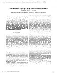
Figure 1. A three-layer perceptron neural network.

Figure 2. A block diagram representation of a three-layer perceptron neural network.

nals propagating along connections and used for the training process. The number of nodes plus the connectivity de® ne the topology of the network, and range from totally connected to a topology where each node is just connected to its neighbours. 3.1. Multi-layer perceptron networks A typical MLP neural network with an input layer, an output layer, and two hidden layers is shown in Fig. 1. For convenience, the same network is denoted in block diagram form as shown in Fig. 2 with three weight matrices W 1, W 2 and W 3 and a diagonal non-linear operator C with identical sigmoidal elements g following each of the weight matrices.1 Each layer of the network can then be represented by the operator

[]

[

]

( 1)

[ W 3C [ W 2C [ W 1x] ] ] = N3N2N1[x].

( 2)

Ni x = C W i x , and the input-output mapping of the MLP network can be represented by

[]

y = Nx = C

The weights of the network W 1, W 2 and W 3 are adjusted (as described in § 3.2) to minimize a suitable function of error e between the predicted output y of the network and a desired output yd (error-correction learning), resulting in a mapping function Nx. It has been shown in Hornik et al. (1988), using the Stone-Weierstrass theorem, that even an MLP network with just one hidden layer and arbitrarily large number of nodes can approximate any continuous function f ÎC( RN, RM) over a compact subset of RN to arbitrary precision (universal approximation). This provides the motivation to use MLP networks in modelling/identi® cation of any manufacturing process’ response characteristics.

[]

1

The most popular non-linear nodal function for perceptron networks is the sigmoid

[unipolar ® f (x) = 1 /(1 + e- x) and bipolar ® f (x) = ( 1 - e- x) /(1 + e- x)].

2604

R. B. Chinnam and W. J. Kolarik

3.2. Back-propagation in ML P networks If MLP networks are used to solve the identi® cation problems treated in this paper, the objective is to determine an adaptive algorithm or rule which adjusts the weights of the network based on a given set of input-output pairs. An error-correction learning algorithm will be discussed here, and readers can see Zurada (1992) and Haykin (1994) for information regarding other training algorithms. If the weights of the networks are considered as elements of a parameter vector µ, the error-correction learning process involves the determination of the vector µ* which optimizes a performance function J based on the output error. In error-correction learning, the weights are adjusted along the negative gradient of the performance function as follows: µ( s+ 1) = µ( s)

-

J( s) h ¶ ( s) ¶µ

( 3)

where h is a positive constant that determines the rate of learning and the superscript refers to the iteration step. In the literature, a well-known method for determining this gradient for MLP networks is the back-propagation method, which is not repeated here. For further information, see Haykin (1994). 3.3. Radial basis function neural networks MLP neural networks have been widely studied and used for approximating arbitrary functions of a ® nite number of real variables (Park and Sandberg 1991). However, traditional training algorithms such as back-propagation require long computation times for training. Also, the incremental adaptation approach of back-propagation can be shown to be susceptible to false minima (Specht 1990). It has been proven that feed-forward networks that incorporate radial basis functions as nodal functions ( RBF networks) are capable of universal approximation with one hidden layer (Park and Sandberg 1991) and can be trained more rapidly (Moody and Darken 1989). For further information regarding the comparison of RBF networks and MLP networks, see Haykin (1994). A typical RBF network consists of three layers of nodes with successive layers fully connected by feed-forward arcs, as shown in Fig. 3. The connections between the input and the hidden layers are unweighted, and the transfer functions at the

Figure 3. A typical radial basis function network.

Neural network-based quality controllers

2605

hidden layer nodes are radial basis functions. Many di€ erent architectures are popular in the literature. Here, the particular architecture and training scheme described in Moody and Darken (1989) is presented along with a transfer function similar to the multivariate Gaussian density function: ¹ ah = e( - i X- h i

2

/sh ) 2

, h = 1, . . . , H,

( 4)

where ah is the output of node h in the hidden layer given the input vector X. Each RBF node has N + 1 internal parameters: mh , the position of the centre of the radial unit in the input space, and sh , the unit width. Each RBF unit has a signi® cant activation over a speci® c region determined by mh and sh . The value of the ith output node, yi , is given by H+ 1

yi =

åw a , i = 1, . . . , M. ih h

( 5)

h= 1

A bias node is represented by aH+ 1 = 1. A three-step polynomial time method presented in Moody and Darken (1989) is generally used to determine the parameters mh , sh , and wih. First, unit centres mh are determined by k-means clustering (MacQueen 1967). Then, a P-nearest neighbour heuristic is used to determine the unit widths sh . Finally, second-layer weights are determined by linear least-squares. For further information regarding the theory, design and application of radial basis function networks, see Haykin (1994), Broomhead and Lowe (1988), Moody and Darken (1989), Renals (1989), and Poggio and Giroski (1990). 4. Proposed approach to design of intelligent quality controllers In order to implement an intelligent quality controller, traditional approaches need to incorporate the following three features: (1) an ability to track changes in process response characteristics with time, (2) an ability to monitor uncontrollable variables, and (3) an ability to perform real-time process parameter design. The conceptual design of such a controller that has shown promise is described herein. Figure 4 illustrates the proposed structures of such an intelligent quality controller. In contrast to the classical approach, this structure includes two distinct feedback control loops. The process control loop `maintains’ the controllable variables at the optimal levels. It is the quality controller in the quality control loop that `determines’ these optimal levels. The quality controller includes both a nonpara-

Figure 4. Architecture for the quality controller at the machine level.

2606

R. B. Chinnam and W. J. Kolarik

metric model of the manufacturing process (modelled here by an ANN) and an optimization routine to ® nd the optimal levels of the controllable variables. At di€ erent stages of knowledge about the manufacturing process, the quality controller will require di€ erent information and run di€ erent experiments. These experiments are designed using an experiment planner as indicated in Fig. 4. In solving this real-time process parameter design problem, the following assumptions are made: (1) process response characteristics of interest at any single instant of time can be expressed as non-linear maps in the input space (vector space de® ned by controllable and uncontrollable variables), (2) levels of uncontrollable variables do not change radically, but change in a reasonably smooth fashion, and (3) scales for the controllable variables are continuous. To simplify the design procedure, the quality controller is designed to operate in two distinct modes: (1) an online process identi® cation mode and (2) a real-time process parameter design mode. 4.1. On-line process identi® cation mode During this process identi® cation mode, the quality controller will repeatedly go through the following stages: (1) identi® cation of signi® cant process response characteristics (depending on the formal objectives of the process designer), (2) identi® cation of both controllable and uncontrollable variables that have signi® cant in¯ uence on the process response characteristics, and (3) model building. Begining with approximate estimates (given by process designers and/or operators), nonparametric/empirical models (using ANNs) are built which relate each process response characteristic of interest with signi® cant controllable and uncontrollable variables in the control domain through structured experimentation and on-line data, to the desired level of accuracy. Let X = ( X1, . . . , XK, Xk+ 1 , . . . , XN) T be a column vector of K controllable variables, X1 through Xk , and N - K uncontrollable variables (noise factors), XK+ 1 through XN, where K £ N. Let Y = ( Y 1 , . . . Y M) T be a vector of M process response characteristics of interest. Traditionally the process response characteristic vector Y is treated as a function of X1 through XN, and takes the form: Y = f ( X), ( 6) in time-invariant systems. As mentioned earlier, most manufacturing systems are time-variant systems, and hence, call for modelling Y as a function of X and time t, taking the form Y = f ( X, t). ( 7) Currently, there is no universal procedure to arrive at the desired function f ( X, t). In manufacturing systems, it is unlikely that a single stochastic model could describe the system’s response characteristics over all points in time t (the past, the present, and the future). However, to solve the real-time process parameter design problem, it would su ce if we could approximate f from (7) with the following empirical model: ~

f ( X) < f (X, t)|t = t0,

( 8)

such that ~

JIdentification = i f ( X) - f ( X, t)i

Identification

£²

( 9)

2607

Neural network-based quality controllers

for some speci® ed constant e ³ 0 and a suitably de® ned norm (denoted by i . i Identification), at all instants in real-time t =~ t0. In other words, it is su cient to update the system’s functional relationship f in real-time, and utilize the levels of uncontrollable variables at t0 to determine the optimal levels for controllable variables for the immediate future. 4.2. Real-time process parameter design mode Once the process identi® cation is completed, the system can be optimized in real~ d T ) denote the vector of M time using the process model, f ( X). Let Yd = ( Y 1d , . . . , Y M desired/target process response characteristics of interest. The objective is to determine the optimal levels for the K controllable variables, X1 through XK, to minimize JParameterDesign = i Y - Yd i ParameterDesign = i f ( X, t) - Yd i ParameterDesign ,

( 10)

for a suitably de® ned norm (denoted by i . i ParameterDesign) on the output space, at all instants in real-time t = t0. In (10), f ( X, t) denotes the output of the process and hence f ( X, t) - Yd º ed is the di€ erence between the process output and the desired output Yd . In the absence of any knowledge about f ( X, t), the objective is to minimize the performance criterion JParameterDesign = i Y - Yd i

ParameterDesign

~ = i f ( X) - Yd i

ParameterDesign

,

( 11)

at all instants in real-time. The constraints would be those restricting the levels of the controllable variables to an acceptable domain. 5. Technical design of the quality controller Section 5.1 introduces the means and methods of performing process identi® cation using MLP and RBF networks and § 5.2 introduces the means and methods of performing process parameter design. 5.1. Process identi® cation It is clear from previous discussion that both MLP networks (with a non-linear nodal function such as the sigmoid) and RBF networks are capable of approximating any continuous function f ÎC( RN, RM) over a compact subset of RN. This result (that both these types of networks are capable of universal approximation) provides the motivation to assume that the non-linear maps generated by these networks are adequate to model the process response characteristics of manufacturing systems at any point in time. Training information can be obtained by observing the input± output behaviour of the process, as suggested in Fig. 5. Here, the network receives the same input signals as the process, and the process response characteristics are used as the target network output. The network topology has to be selected in such a fashion that generalization (extrapolation to novel instances being e€ ective) is maintained. Several guidelines are discussed in the literature, which are not repeated here (Weigand et al. 1992, Denker et al. 1987, Solla 1989, Baum and Haussler 1989). The standard procedures for adjusting the network parameters are discussed in §§ 3.2 and 3.3 for MLP networks and RBF networks, respectively.

2608

R. B. Chinnam and W. J. Kolarik

Figure 5. Using a neural network for process identi® cation.

5.2. Process parameter design This section introduces an iterative inversion method to determine the optimal controllable variable levels for the process in real-time. This approach utilizes the trained ANN that resulted from the previous identi® cation phase. In error back-propagation training of neural networks, the output error is `propagated backward’ through the network. Linden and Kinderman (1989) have shown that the same mechanism of weight learning can be used to iteratively invert a neural network model. In this approach, errors in the network output are ascribed to errors in the network input signal, rather than to errors in the weights. Thus, iterative inversion of neural networks proceeds by a gradient descent search of the network input space (spanned by controllable and uncontrollable variables), while error back-propagation training proceeds through a search in the synaptic weight space. Through iterative inversion of the network, one can generate the optimal controllable variable input vector, X1 , . . . , XK , that gives an output as close as possible to the desired process performance characteristics of interest. By taking advantage of the duality between the synaptic weights and the input activation values in minimizing the performance criterion, JParameterDesign, the iterative gradient descent algorithm can again be applied to obtain the desired input vector:

[

( s+ 1)

Xj

( s)

= Xj

]

J ( s) + a( Xj - h ´ ¶ ParameterDesign ( s)

¶Xj

( s 1) Xj - ).

( 12)

Here the superscript refers to the iteration step, h and a are the rates for the learning and momentum in the gradient descent approach. Here the least means square criterion was used as the performance criterion. In that case, for the three-layered MLP network shown in Fig. 1, the gradient of the performance criterion with respect to the controllable variable Xj , ¶J /¶Xj can be shown to be as follows:

å[

O ¶J = M ( Y d ( ) ) Y Y 1 Y m m m ¶Xj m= 1 m q= 1

{

´ Wme ´q ´ Zq( 1 - Zq) ´

å

P

å[ W p= 1

2 q´p

´ V p( 1 - V p) ´ Wp1´j ]

}]

.

( 13)

For the RBF network shown in Fig. 3, the gradient of the performance criterion with respect to the controllable variable Xj , ¶J /¶Xj , can be shown to be as follows:

2609

Neural network-based quality controllers

¶J =¶Xj

å[ M

m= 1

( Y m - Y md )

{

H

åW h= 1

2 mh

[ ah ´ {2( Xj ´ Whj1 -

Mhj ) } ´ Whj1 ]

}]

.

( 14)

The readers are referred to Chinnam (1994) for the derivations of these gradients. 6. Performance evaluation of the proposed quality controllers Each manufacturing process is di€ erent by its very nature, but from a statistical point of view many similarities exist. These similarities allow development of a simulation based test-bed, useful for qualitative assessment of both the bene® ts and burdens associated with experimental based strategies such as quality controllers and experimental designs. A test-bed, named ProtoSim, was developed by the authors to simulate pre-de® ned but hypothetical process response characteristics of manufacturing processes. In the absence of ® rst-principle cause± e€ ect models for the particular process of interest, empirical models developed from physical experimentation results provide the means for emulation. ProtoSim has the ability to emulate non-stationary processes with complex non-linearities and interactions, and allows evaluation of process quality controllers by providing interaction between the process simulator and the quality controller, as illustrated in Fig. 6. Once provided with the information regarding the particular process of interest, ProtoSim prompts the user to select the desired quality controller model, as depicted in Fig. 7. ProtoSim works with two types of quality controller models that depend on MLP networks and RBF networks for process identi® cation, respectively. After the selection of the desired quality controller model and the patterns/signatures followed by the uncontrollable variables, ProtoSim starts simulating the manufacturing process and the respective uncontrollable variables. The selected quality controller model starts acquiring/extracting information regarding the process response characteristics from the simulator by conducting designed experiments (currently the

Figure 6. Simulator acting as a test-bed for quality controllers.

2610

R. B. Chinnam and W. J. Kolarik

Figure 7. Layout of the simulator.

quality controller is equipped to conduct experiments using full factorial designs only). The quality controller upon conducting the experiments moves into the process identi® cation mode (and starts training the ANNs using the training vectors obtained through the experiments). Whenever it is time to determine the levels for the controllable variables (depends on the information provided by the user as part of the system speci® cation), the quality controller temporarily moves from the process identi® cation mode into parameter design mode, and suggests `optimal’ levels for the controllable variables. 6.1. Flow of control during identi® cation mode Structural learning in ANNs, de® ned as the process of determining the class of neural network models most applicable for a particular application (Barto 1991), is critical in on-line process identi® cation. In quality controllers that incorporate multilayer perceptron networks, structural learning involves the number of layers, number of hidden units, and kinds of constraints that should be used. In quality controllers that utilize RBF networks, this learning involves the number of RBF centres and parameters associated with the nodal function used. To achieve good generalization, ProtoSim initializes the neural network used for process identi® cation with the fewest number of parameters. Then, the number of parameters are incremented until the desired level of accuracy is attained, as depicted in Fig. 8. ProtoSim incorporates features to handle partially connected networks, as well as generalization enhancement techniques such as weight elimination proposed by Weigand et al. (1992) and S-fold cross-validation proposed by Weiss and Kulikowski (1991). 6.2. Flow of control during parameter design mode In searching for optimal controllable variable levels, ProtoSim incorporates iterative inversion with respect to the energy surface in the input domain. ProtoSim, by default, de® nes the energy function as the least-squares di€ erence between the

Neural network-based quality controllers

2611

Figure 8. Flow of control in process identi® cation mode.

desired performance characteristics and the predicted performance characteristics with respect to the controllable and uncontrollable variables levels. If the energy function meets all the criteria for a strictly convex function in the input domain, gradient descent techniques lead to a global optimal solution. However, if the energy function is not a convex function, gradient descent techniques by de® nition lead to a local optimal solution. Hence, it is necessary that the quality controllers search through all the basins (multiple basins might exist in the case of non-convex energy functions) to locate the global optimal levels for the controllable variables. Currently, the quality controllers implemented along with ProtoSim lack the ability to locate global optimal solutions. The solution depends on the location of the starting point in the input domain from which the search process was initiated. Under the assumption that the step sizes taken along the negative gradient are not large enough to move into a di€ erent basin, the quality controller converges to the local minimum in the basin holding the starting point. However, it is easy to incorporate a simulated annealing module (or other enhanced optimization techniques) to converge towards a global optimal solution. This search process is illustrated in Fig. 9. 6.3. Experimental evaluation of the proposed quality controller models on ProtoSim Software constraints posed by the graphic user interface (GUI) has restricted the ¯ exibility of ProtoSim to allow for the simulation of processes having a maximum of two uncontrollable variables, two controllable variables, and two response characteristics. To evaluate the e€ ectiveness of the MLP and RBF quality controllers, several production processes had been simulated on ProtoSim. These simulations were designed and executed with various kinds of process response characteristics. The following section provides a detailed discussion about a speci® c simulation of a printing machine used for applying colouring ink package labels.

2612

R. B. Chinnam and W. J. Kolarik

Figure 9. Flow of control in parameter design mode.

6.3.1. An experiment for evaluation of quality controllers An experiment was designed to evaluate the performance of an RBF quality controller model. This experiment tested the quality controller performance in the identi® cation mode as well as the process parameter design mode. The models of the process response characteristics of the printing machine were obtained from Castillo and Montgomery (1993). The objective is to optimize the controllable variables, speed (denoted by X2 ) and pressure (denoted by X3 ), from time-to-time to re¯ ect changes in the uncontrollable variable distance (denoted by X1 ). Two process response measures were of interest and their respective models are as follows: ReasMeas1 ( X) = 327´6 + 131´5X1 + 177´0X2 + 109´4X3 - 29´1X12 + 32´0X22

-

22´4X32 + 75´5X1X2 + 43´6X1X3 + 66´0X2 X3 ,

-

1´3X32 + 5´1X1 X2 + 14´1X1 X3 + 7´7X2X3 ,

ResMeas2 ( X) = 34´9 + 29´2X1 + 11´5X2 + 15´3X3 + 16´8X12 + 4´2X22 where - 1 £ Xi £ + 1; i = 1, 2, 3.

Neural network-based quality controllers

Figure 10.

2613

Response surfaces of a simulated process. (a) Surface for ResMeas1( X). (b) Surface for ResMeas2( X).

These response characteristics of the printing machine are illustrated in Fig. 10. Please note that the response measure values have been scaled using a unipolar sigmoid function, f ( x) = 1 /( 1 + exp( - ¸x)), to limit the values between 0´0 and 1´0. The scaling factor, ¸, was chosen to be 0´01. This scaling is necessary to ensure that the data is ready for training both MLP networks or RBF networks used in the quality controller. In particular, MLP networks with sigmoid nodal functions in the output layer nodes call for such scaling. 6.3.2. Quality controller performance in the identi® cation mode Initially, a three-level factorial experiment was conducted by the quality controller, resulting in 27 observed data sets serving as training patterns for the process

2614

R. B. Chinnam and W. J. Kolarik P

10 9 8 7 H

6 5 4 3 2

1

2

3

4

5

6

7

8

9

7´94 5´09 6´45 4´32 7´44 4´93 7´39 4´27 6´17 4´25 7´16 4´26 7´39 3´77 9´40 6´10 10´40 7´05

6´71 5´28 5´17 3´81 7´11 3´83 7´06 4´00 5´95 3´84 7´01 4´12 6´87 3´53 10´40 6´12

6´39 4´22 5´22 2´78 5´77 2´86 6´71 3´66 5´76 3´58 6´75 3´89 6´23 4´67

6´36 3´42 5´74 2´48 5´58 2´53 6´63 3´41 5´66 3´47 5´52 3´83

6´40 3´12 5´57 2´21 5´51 2´28 6´76 3´45 5´34 3´63

6´50 2´72 5´70 2´09 5´56 2´13 6´05 3´94

6´47 2´58 6´24 1´98 5´89 2´91

6´83 2´26 5´63 1´18

7´13 4´72

All entries were scaled by a factor of 100. The ® rst and second cell entries refer to the MSEs corresponding to the ® rst and second response measures respectively. Table 1. The MSE values corresponding to various combinations of H and P; three-level factorial experiment.

identi® cation mode of the quality controller. The levels for each of the three independent variables were chosen as - 1, 0, and + 1 by the quality controller.2 At ® rst, the optimal values for the identi® cation network parameters H and P were determined using the 5-fold cross-validation procedure (Weiss and Kulikowski 1991).3 The possible values for H and P ranged from 2 to 22 and 1 to 21, respectively. The MSE values of the RBF network training error corresponding to various combinations of H and P are provided in Table 1. The performance criterion considered for determining the optimal values of the parameters H and P to be 9 and 8 respectively. The level of prediction accuracy yielded by the RBF network structure having the above determined parameter values was found to be highly unacceptable, as depicted in Fig. 11. Attributing this lack of prediction accuracy to an inadequate number of training patterns, the quality controller resorted to a four-level factorial experiment. The factor levels were again selected by the controller in such a manner that they were uniformly spaced in the input domain. The MSEs corresponding to the two response measures are provided in Table 2 for various combinations of H and P. Once again, using the same 5-fold crossvalidation procedure, the optimal values of the identi® cation structure parameters H and P were selected by the quality controller as 18 and 19, respectively. These new 2

It must be noted that the level of uncontrollable variable was zero for all the response surfaces that were illustrated for this particular experiment. 3 Since there are relatively few training patterns (just 27), 5-fold cross-validation would be appropriate, allowing 80% of the training data set (i.e., ( 5 - 1) /5 of 27 is approximately 22 training patterns) to be used for training and the remaining 20% (i.e., 1 /5 of 27 is 5 training patterns) for evaluation during each cross-validation loop, and there will be 5 loops in total.

Neural network-based quality controllers

2615

Figure 11. Predicted and actual response surfaces of a simulated process; three level factorial experiment. (a) Predicted surface for ResMeas1( X) superimposed on the actual surface. (b) Predicted surface for ResMeas2( X), superimposed on the actual surface. (c) Error surface.

parameters yielded a 2-fold improved prediction accuracy in comparison with the three-level factorial experiment, as depicted in Fig. 12. Having achieved the desired level of accuracy (provided to ProtoSim as part of user speci® cation), the quality controller shifted from the current identi® cation mode to process parameter design mode. 6.3.3. Quality controller performance in the parameter design mode The e€ ectiveness of the quality controller in the parameter design mode was tested under a number of possible combinations of starting points4 and desired 4

Starting point defines the values of the controllable variables in the input domain at the time the desired targets were provided to the quality controller in the parameter design mode.

2616

R. B. Chinnam and W. J. Kolarik P 1 20 18 16 14

H

12 10 8 6 4 2

3

5

5´09 3´37 3´02 2´89 1´59 1´33 5´54 4´27 3´60 2´69 1´76 1´45 5´08 4´08 3´68 2´36 1´81 1´35 5´39 52´80 14´70 2´64 39´50 11´40 4´86 3´60 2´89 2´76 1´96 1´38 4´49 4´32 4´17 2´47 2´12 1´66 4´24 3´75 3´44 2´21 2´02 1´71 5´13 4´61 3´89 3´23 2´69 2´41 5´71 5´02 3´48 3´35 8´47 6´21

7

9

11

2´57 2´55 2´44 0´98 0´82 0´64 2´87 2´50 2´31 1´04 0´84 0´68 2´85 2´78 2´44 0´99 0´74 0´17 3´07 17´80 13´8 1´12 13´20 15´8 2´63 2´46 2´83 1´06 0´87 0´78 4´00 3´29 1´28 0´96 3´53 1´61

13

15

17

19

2´56 0´66 2´48 0´61 2´59 0´57 2´97 0´47

2´49 0´54 2´45 0´50 2´80 0´55

3´00 1´01 2´60 0´67

3´21 1´65

All entries were scaled by a factor of 100. The ® rst and second cell entries refer to the MSEs corresponding to the ® rst and second response measures respectively. Table 2. The MSE values corresponding to various combinations of H and P; four-level factorial experiment.

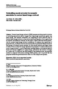
process response measure targets. For illustrative purposes, the results corresponding to two combinations shown in Table 3 are discussed here. For Case 1, the quality controller in the parameter design mode was successful in converging to an optimal solution within the basin as shown in Fig. 13. The white bullet corresponds to the starting point and the connected black bullets depict the gradient descent trajectory followed by the search process. The energy surface shown in Fig. 13 indicates that the search process yielded optimal values for the controllable variables (a state of zero energy). The other case reiterated the same convergence phenomena discussed for Case 1. The response surface corresponding to Case 2 is shown in Fig. 14. Based on the various tests conducted to evaluate the e€ ectiveness of both quality controllers, the following observations are made: (1) as expected, the energy surface changes with changing desired target values, (2) the starting point greatly in¯ uences the search process, and (3) the search process guaranteed optimal solutions within the basin of attraction. 6.3.4. Overall performance evaluation results Based on the results from the process simulation test-bed, it was observed that both the MLP and RBF quality controllers performed extremely well in building e€ ective nonparametric models of the manufacturing processes. Both the MLP network based iterative-inversion and the RBF network based iterative-inversion approaches were extremely consistent in converging towards optimal solutions within the basin of attraction.

2617

Neural network-based quality controllers

Figure 12. Predicted and actual response surfaces of a simulated process; four level factorial experiment. (a) Predicted surface for ResMeas1( X) superimposed on the actual surface. (b) Predicted surface for ResMeas2( X) superimposed on the actual surface. (c) Error surface.

Starting point Uncontrollable variable

Case 1 Case 2

Controllable variables

Target values

X1

X2

X3

Resmeas1( X )

Resmeas2( X )

0´000 0´000

0´000 0´000

0´850 0´850

0´930 0´817

0´570 0´549

Table 3. Combinations of starting points and desired targets.

2618

R. B. Chinnam and W. J. Kolarik

Figure 13. Energy surface with superimposed search trajectory (Case 1). Desired targets at 0´93 and 0´57; starting points at X2 = 0´0, X3 = 0´85.

7. Conclusion In contrast to classical on-line and o€ -line quality assurance procedures that are compatible with open-loop process control, the concept of a closed-loop quality controller was introduced. The work presented can be best characterized as an investigation of neural networks for e€ ective process identi® cation and real-time process parameter design of manufacturing systems. The identi® cation function involves development of nonparametric/empirical models relating controllable and uncontrollable variables to process response characteristics of interest. Two general classes of identi® cation structures have been introduced to perform the identi® cation function using MLP and RBF neural networks, respectively. The developed identi® cation structures have been tested on several simulated production processes, and were observed to be extremely successful in building models.

Neural network-based quality controllers

2619

Figure 14. Energy surface with superimposed search trajectory (Case 2). Desired targets at 0´817 and 0´549; starting points at X2 = 0´0, X3 = 0´85.

The process parameter design function involves usage of the identi® ed process models and the levels of the uncontrollable variables, to provide levels for the controllable parameters that will lead to the desired levels of the quality characteristics in real-time. An iterative neural network inversion approach is introduced to search the parameter space for determining optimal levels for the controllable variables. The proposed quality controllers when tested on a simulation test-bed proved to be extremely successful in performing process parameter design. This work represents a ® rst step in this direction and future research work would involve the application of these intelligent quality control methods to di€ erent classes of manufacturing systems/processes and the study of issues involved in the integration of this approach with model based control approaches and other process control approaches.

2620

Neural network-based quality controllers

Acknowledgments The authors are very grateful for the detailed comments and suggestions by two referees. Their contributions have led to substantial improvements in the contents and presentation of this paper. Research funding by the North Dakota EPSCoR/ NSF program and the State of Texas under the ARP/ATP program is greatly acknowledged. References Barto , A. G., 1991, Neural Networks for Control (Cambridge, MA: MIT Press). Baum, E. B. and Hau ssler , D., 1989, What size net gives valid generalization? Neural

Computation, 1, 151± 160.

Broomhea d , D. S. and Lowe, D., 1988, Multivariable functional interpolation and adaptive

networks. Complex Systems, 2, 321± 355.

Box , G. E. P. and Wilson , K. B., 1951, On the experimental attainment of optimum condi-

tions. Journal of Royal Statistical Society, B13, pp. 1± 38.

Chinna m, R. B., 1994, Intelligent Process Quality Control and Tool Monitoring in

Manufacturing Systems. PhD thesis, Texas Tech University, Lubbock, TX, USA.

Castillo , E. D. and Montgomery , D. C., 1993, A nonlinear programming solution to the

dual response problem. Journal of Quality Technology, 25, 199± 204.

Denker , J. S., Schwartz , D. B., Wittner , B. S., Solla , S. A., Howard , R. E., Jackel , L. D. and Hopfield , J. J., 1987, Automatic learning, rule extraction, and generaliza-

tion. Complex Systems, 1, 877± 922.

Haykin , S., 1994, Neural Networks: A Comprehensive Foundation (New York: Macmillan). Hornik , K., Stinchcombe , M. and White, H., 1988, Multi-layer feed-forward networks are

universal approximators. Discussion paper, Dept. of Economics, University of California, San Diego, CA. Kacker , R. N., 1985, O€ -line quality control, parameter design, and the Taguchi method. Journal of Quality Technology, 17, 176± 209. Linden, A. and Kindermann , J., 1989, Inversion of multi-layer nets. Proceedings of the International Joint Conference on Neural Networks, Washington, DC, pp. 425± 430. Lippma n, R. P., 1987, An introduction to computing with neural nets. IEEE ASSP Magazine, 4± 22. Mac Queen , J., 1967, Some methods for classi® cation and analysis of multivariate observations. Proceedings of the 5th Berkeley Symposium on Mathematical Statistics and Probability, Berkeley, CA, pp. 281± 297. Moody , J. and Darken, C. J., 1989, Fast learning in networks of locally tuned processing units. Neural Computation, 1, 281± 294. Myer s, R. H. and Carter , W. H. Jr ., 1973, Response surface techniques for dual response surfaces. Technometrics, 15, 301± 317. Park , J. and Sandber g , I. W., 1991, Universal approximation using radial-basis-function networks. Neural Computation, 3, 246± 257. Poggio , T. and Giroski, F., 1990, Networks for approximation and learning. Proceedings of the IEEE, 78, 1481± 1497. R enals , S., 1989, Radial basis function network for speech pattern classi® cation. Electronics L etters, 25, 437± 439. Solla , S. A., 1989, Learning and generalization in layered neural networks: the contiguity problem. In Neural Networks from Models to Applications, Dreyfus, G. and Personnaz, L. (eds) (Paris: IDSET), pp. 168± 177. Specht , D. F., 1990, Probabilistic neural networks. Neural Networks, 3, 109± 118. Weiga nd , A. S., R umelhart , D. E. and Huberman , B. A., 1992, Advances in Neural Information Processing Systems (San Mateo, CA: Morgan Kaufmann). Weiss, S. M. and Kulik owski, C. A., 1991, Computer Systems That L earn (San Mateo, CA: Morgan Kaufmann). Zurada , J. M., 1992, Introduction to Arti® cial Neural Systems (St. Paul, MN: West Publishing).