European Journal of Scientific Research ISSN 1450-216X Vol.33 No.1 (2009), pp.163-178 © EuroJournals Publishing, Inc. 2009 http://www.eurojournals.com/ejsr.htm
New Supervised Multi Layer Feed Forward Neural Network Model to Accelerate Classification with High Accuracy Roya Asadi Faculty of Computer Science and Information Technology University Putra Malaysia, 43400 Serdang, Selangor, Malaysia E-mail:
[email protected] Norwati Mustapha Faculty of Computer Science and Information Technology University Putra Malaysia, 43400 Serdang, Selangor, Malaysia E-mail:
[email protected] Nasir Sulaiman Faculty of Computer Science and Information Technology University Putra Malaysia, 43400 Serdang, Selangor, Malaysia E-mail:
[email protected] Nematollaah Shiri Dept of Computer Science and Software Engineering Concordia University, Montreal, Canada E-mail:
[email protected] Abstract The main problem for Supervised Multi-layer Neural Network (SMNN) model such as Back propagation network lies in finding the suitable weights during training in order to improve training time as well as achieve high accuracy. The important issue in the training process of the existing SMNN model is initialization of the weights which is random and creates paradox, and leads to low accuracy with high training time. In this paper, a new Supervised Feed Forward Multi-layer Neural Network (SFFMNN) model for classification problem is proposed. It consists of a new preprocessing technique which combines data preprocessing and pre-training that offer a number of advantages; training cycle, gradient of mean square error function, and updating weights are not needed in this model. In new SMFFNN model, thresholds of training set and test set are computed by using input values and potential weights. In training set each instance has one special threshold and class label. In test set the threshold of each instance will be compared with the range of thresholds of training set and the class label of each instance will be predicted. To evaluate the performance of the proposed SMFFNN model, a series of experiment on XOR problem and two datasets, which are SPECT Heart and SPECTF Heart was implemented with 10fold cross-validation. As quoted by literature, these two datasets are difficult for classification and most of the conventional methods do not process well on these datasets. Our results, however, show that the proposed model has been given high accuracy in one epoch without training cycle.
New Supervised Multi Layer Feed Forward Neural Network Model to Accelerate Classification with High Accuracy
164
Keywords: SMNN, SMFFNN, Training, Epoch, Preprocessing, Pre-training
1. Introduction Learning is the important property of neural networks. Neural networks are able to dynamically learn types of input information based on their weights and properties. During learning, the weight of each value in hidden layers will be considered. As the domain becomes smaller and smaller, suitable weights will be obtained through this series of repeated trial and errors after several epochs. Suitable data pre-processing techniques are necessary to find input values while pre-training techniques to find desirable weights that in turn will reduce the training process. This is the essence of Supervised Multilayer Neural Network (SMNN). Usually preprocessing is applied for helping improve the accuracy, speed and scalability of the classification. Without preprocessing, the classification process will be very slow and it may not even complete (Han and Kamber, 2001). Currently, data preprocessing and pre-training are main ideas in developing efficient techniques for fast SMNN processing, high accuracy and reducing the training process (Van der Maaten et al., 2008; Hinton and Salakhutdinov, 2006) but the problems in finding the suitable input values and the suitable weights, processing time and high accuracy are still remain (Demuth et al., 2007; Andonie and Kovalerchuk, 2004; Jolliffe, 2002; Han and Kamber, 2001). The current pre-training techniques generate suitable weights for reducing the training process but applying random values for initial weights (Van der Maaten et al., 2008; DeMers and Cottrell, 1993) and this will create paradox (Zhang et al., 2003; Fernández-Redondo and Hernández-Espinosa, 2001). In this paper, we proposed a new preprocessing technique that is combination of data pre-processing and pre-training in SMNN results in worthy input values, desirable process, and higher performance in both speed and accuracy. The rest of this paper is organized as follows: In section 2, we discuss about the backpropagation network method and review some related works in preprocessing and pre-training techniques used in BPN. Section 3 describes the proposed technique for preprocessing and the new SMFFNN that using the proposed technique is discussed in Section 4. Finally, the experimental results and conclusion with future works are reported in Section 5 and Section 6 respectively.
2. Previous Research Since our work used BPN as one of SMNN model, here we describe about the BPN and its preprocessing and pre-training techniques has been done to increase the performance in terms of speed and accuracy for classification problem. 2.1. Back-propagation network Back-propagation network (BPN) (Werbos, 1974) is the best example of a parametric method for training supervised multi-layer perception neural network for classification. BPN like other SMNN models has the ability to learn biases and weights (Han and Kamber, 2001). It is a powerful method to control or classify systems that use data to adjust the network weights and thresholds for minimizing the error in its predictions on the training set. Learning in BPN employs gradient-based optimization method in two basic steps: to calculate the gradient of error function and to compute output by the gradient. Also, BPN compares each output value with its sigmoid function in the input forward and computes its error in BPN backward. This is considerably slow because biases and weights have to be updated in each epoch of learning (Mark and Jude, 1997). Pre-processing in real world environment focuses on data transformation, data reduction, and pre-training. Data transformation and normalization are two important aspects of pre-processing. Transformation data is codification of values of each row in input values matrix and changing them to one data. Data transformation often uses algebraic or
165
Roya Asadi, Norwati Mustapha, Nasir Sulaiman and Nematollaah Shiri
statistical formulas. Data normalization data transforms one input value to another suitable data by distributing and scaling. Data reduction such as dimension reduction and data compression are applied minimizing the loss of information content. Currently, data pre-processing and pre-training are the contributing factors in developing efficient techniques for fast SMNN processing at high accuracy and reduced training time (Van der Maaten et al., 2008; Hinton and Salakhutdinov, 2006). Figure 1 illustrates the feature of BPN by using data preprocessing and pre-training: Figure 1: Back propagation network by using preprocessing
2.2. Data preprocessing There are several powerful data preprocessing mathematical and statistical functions which are ordinal basis of improving efficiency (Demuth et al., 2007) and will be discussed as current methods in this study. 2.2.1 MinMax as preprocessing Neal et al. (1994) explained about predicting the gold market including an experiment on scaling the input data. MinMax technique will be used in BPN to transform and to scale the input values between 0 and 1 if the activation function is used the standard sigmoid and -1 to 1 for accelerating process (Han and Kamber, 2001; Russell, 2007). The technique of using Log (input value) is similar to MinMax for range [0..1]. Another similar method is Sin( Radian(input value) ) between - π to π where Radian(input value) be between 0 to π (Demuth et al., 2007). Disadvantage of MinMax technique is lack of one special and unique class for each data (LeCun et al., 1998). 2.2.2 Dimension data reduction Dimension data reduction method projects high dimensional data matrix to lower dimensional submatrix for effective data preprocessing. We consider Principal Component Analysis (PCA) (Jolliffe, 1986) because of its properties which will be explained in pre-training section and it is known as the best dimension reduction technique until now (Van der Maaten et al., 2008; Shlens, 2005; Daffertshofer et al., 2004; Lindsay, 2002). PCA is a classical multivariate data analysis method that is useful in linear feature extraction and data compression (Van der Maaten et al., 2008; Shlens, 2005; Daffertshofer et al., 2004; Lindsay, 2002). If the dimension of the input vectors be large, the components of the vectors are highly correlated (redundant). In this situation to reduce the dimension
New Supervised Multi Layer Feed Forward Neural Network Model to Accelerate Classification with High Accuracy
166
of the input vectors is useful. The assumption is most information in classification of high dimensional matrix has large variation. In PCA often are computed maximizing the variance in process environment for standardized linear process. The disadvantage of PCA is not to be able to find non linear relationship within input values; therefore these data will be lost. The main disadvantage of PCA and other functions basis on dimension reduction is losing input values. 2.3. Pre-training The number of epochs in training process depends on initial weights, training of BPN includes of activation function in hidden layers for computing weights deeply. Usually initialization the weights in pre-training of BPN are at random. Also the processing time depends on initial values and weights and biases, learning rate, and topology of network (Zhang et al., 2003; Fernández-Redondo and HernándezEspinosa 2001). In the following, several current methods of pre-training for BPN are discussed. 2.3.1 MinMax as pre-training There are several initial weights methods which are current methods even now such as MinMax (Zhang et al., 2003; Fernández-Redondo, and Hernández-Espinosa, 2001). In the methods of MinMax, initial weights is considered in domain of (-a, +a) which computed experimentally. SBPN is initialed random weights in domain [-0.05, 0.05]. There is an idea that initializing with large weights are important (Ho-Sub et al., 1995). The input values are classified in three groups, the weights of the most important inputs initialized in [0.5, 1], the least important initialized with [0, 0.5] and the rest initialized with [0, 1]. The first two groups contain about one quarter of the total number input values and the other group about one half. Another good idea was introduced for initializing weight range in domain of [−0.77; 0.77] with fixed variance of 0.2 and obtained the best mean performance for multi layer perceptrons with one hidden layer (Keeni et al., 1999). BPN with initialization of weight in [0.05, 0.05] was implemented on HEART and BUPA datasets from UCI repository (FernándezRedondo and Hernández-Espinosa, 2001). Generalization performance was measured by computing the percentage correct with the test set. In HEART or Heart Disease dataset mean value of the percentage correct with the test set is 81.2±1.1 with 220±80 epochs and in BUPA or Liver Disorders mean value of the percentage correct with the test set is 59.4±1.0 with 1300±400 epochs. These results can be compared with pre-training method of SCAWI. We consider initial random weights in range of [-0.77, 0.77] for standard BPN in experiment results. The disadvantage of the method of MinMax is usage of initialization with random numbers which create critical in training. 2.3.2 SCAWI The method called Statistically Controlled Activation Weight Initialization (SCAWI) was introduced in (Drago and Ridella, 1992). They used the meaning of paralyzed neuron percentage (PNP) and concepted on testing how many times a neuron is in a completed situation with acceptable error. The formula of Wij input = 1.3 / (1+N input.V2)1/2. rij is for initializing weights W that V is the mean squared value of the inputs and rij is a random number uniformly distributed in the range [-1, +1]. This method was improved to Wij hidden = 1.3 / (1+0.3. N hidden)1/2. rij for earning better result (Fernandez-Redondo and Hernandez-Espinosa, 2000; Funahash, 1989). BPN by using SCAWI method was implemented on HEART and BUPA datasets from UCI repository too (Fernández-Redondo and Hernández-Espinosa, 2001). In HEART or Heart Disease dataset mean value of the percentage correct with the test set is 80.8.2±1.0 with 200±100 epochs and in BUPA or Liver Disorders mean value of the percentage correct with the test set is 60.9±0.9 with 1600±400 epochs. These results can be compared with pre-training method of MinMax. The speed of BPN by using MinMax pre-training method on HEART dataset is better than the speed of BPN by using SCAWI. The disadvantage of the method of SCAWI is using random numbers to put the formula and it is similar to MinMax method which has critical in training.
167
Roya Asadi, Norwati Mustapha, Nasir Sulaiman and Nematollaah Shiri
2.3.3 Multilayer auto-encoder networks as pre-training Codification is one of five tasks types in neural network applications (Hegland, 2003). Multilayer encoders are feed-forward neural networks for training with odd number of hidden layers (Van der Maaten et al., 2008; DeMers and Cottrell, 1993). The feed forward neural network trains to minimize the mean squared error between the input and output by using sigmoid function. High dimension matrix can reduce to the low-dimensional by extracting the node values in the middle hidden layer. In addition Auto-encoder/Auto-Associative neural networks are neural networks which are trained to recall their inputs. When the neural network uses linear activation functions, auto-encoder processes are similar to PCA (Lanckriet et al., 2004). Sigmoid activation allows to the auto-encoder network to train a nonlinear mapping between the high-dimensional and low-dimensional data matrix. After the pre-training phase, the model is called “unfolded” to encode and decode that initially use the same weights. BPN can use for global fine-tuning phase through the whole auto-encoder to fine-tune the weights for optimization. For high number of multilayer auto-encoders connections BPN approaches are quite slowly. The auto-encoder network is unrolled and is fine tuned by a supervised model of BPN in the standard way. Since the 1980s, BPN has been obvious by deep auto-encoders and the initial weights were close enough to a good result. An auto-encoder processes very similar to PCA (Lanckriet et al., 2004). The main disadvantage of this method is due to the high number of multi-layer autoencoders connections in BPN training process, resulting in slow performance.
3. Hypotheses Based on new Supervised Multi layer Feed Forward Neural Network model to accelerate classification with high accuracy, we test the following hypotheses: H1: Proposed weights linear analysis will increase classification accuracy and reduce training time in the new SMFFNN model. H2: New Supervised Multi-layer Feed Forward Neural Network (SMFFNN) model will increase classification accuracy and improve training time in a single epoch classification.
4. Research Method For estimating the research models and hypothesis testing, we propose new pre-processing technique of weights linear analysis and new SMFFNN model. Finally for illustration of method, the problem of XOR will be considered. 4.1. Hypotheses Testing 4.1.1. Testing proposed WLA to increase classification accuracy and reduce training time in the new SMFFNN model (H1) Proposed technique is Weights Linear Analysis (WLA) for reducing training process and fast classification in new SMFFNN model with high accuracy. The key ideas to propose WLA model are the first to recognize high deviations of input values matrix from global mean similar to PCA and the second pre-training and using the meaning of vector torque formula for New SMFFNN. For data analyzing, the first WLA uses data preprocessing and then uses normalized values for pre-training, at last new SMFFNN can apply normalized input values and their potential weights. The aim of applying WLA technique is to recognize and find which input values have more differences and deviations to global mean similar to PCA technique. These deviations cause more scores for their values. By using the technique of Weights Linear Analysis in New SMFFNN, each normalized value vector creates one vector torque ratio to global mean of matrix. They are evaluated together and they will reach to equilibrium. Figure 2 shows the example of the action for four vector torques, but all vectors create their own vector torques: Figure 2: The action for four vector torques
New Supervised Multi Layer Feed Forward Neural Network Model to Accelerate Classification with High Accuracy
168
Ca, Cb, Cc, Cd are the vectors of values while Da, Db, Dc, Dd are the arms of vector torques of values. These arms are based on their distances from global mean point of matrix. The vector torque of Ca is Ca× Da, the vector torque of Cb is Cb× Db, the vector torque of Cc is Cc× Dc and the vector torque of Cd is Cd× Dd. In this study, the physical and mathematical meaning of vector torque is used, and is used in classification of instances. For example, if vector Ck has much correlation with Ca, by adding to vector torques, it will create noise should the correlation be 1. When correlation is 1, this means that the two attributes are indeed one attribute and duplication exists in input values matrix. Ck that has much correlation with Ca, adds to vector torques, whereby the global mean moves to new location of the torque, closer to location of vector Ca. The vector of Ck correlates with Ca and other vectors, hence after equivalence, the global mean take place as one constant at special point of axis of vector torques. The weight distributed is between Ca and Ck as shown in Figure 3. Figure 3: The action of four vector torques with entrancing new vector
Phases of Weights Linear Analysis: There are three phases in implementing WLA: Input values matrix: The input values can be every numeric type, range and measurement unit. If the dataset is large, there a high chance that the vector components are highly correlated (redundant). Even
169
Roya Asadi, Norwati Mustapha, Nasir Sulaiman and Nematollaah Shiri
though the input values have correlation, hence the input is noisy; WLA method is able to solve this problem. In statistics, the correlation is ρij based on standard deviation σ and covariance Cov. The covariance function returns the average of deviation products for each data value pair two attributes. Data preprocessing phase in WLA: In this phase, data pre-processing performance is considered. The technique of Min and Max is used. Each value is computed to find the ratio to average of all columns. Pre-training phase in WLA: In improving pre-training performance, potential weights are initialized. The first distribution of standard normalized values is computed. μ is mean of values vectors each row, and σ is standard deviation of values vectors each row. Znm is a standard normalized value and is computed based on formula below. Znm = ( Xnm – μm ) /σm We explained the arms of value vectors are computed based on definition of deviation and distribution of standard normalization. Znm shows the distance of Cnm to mean its rows. Global mean is the center of vectors torques. The weights are arms in vectors torques and the distance is global mean of input values matrix. This definition of weight is based on statistical and mathematical definition of normalization distribution and vector torque. Wm is equivalent to |Z11|+|Z22|+|Z…|+|Znm| ) / n. |Znm| is absolute of normal value Znm. Hence, weight selection is not randomization. The weights may have thresholds but must be managed in hidden layer of new SMFFNN using the following equation. Wm = ( |Z11|+|Z22|+|Z…|+|Znm| ) / n The time complexity of WLA technique depends on the number of attributes p and the number of instances n. The technique of WLA is linear and its time complexity will be O(pn). 4.1.2. Testing new SMFFNN model to increase classification accuracy and improve training time in a single epoch classification (H2) WLA technique output normalized input values and potential weights. New SMFFNN will process based on the algebraic consequence of vectors torques. The vectors torque Tnm = Cnm × Wm are the basis of the physical meaning of torque. Each torque T shows a real worth of each value between whole values in matrix. The algebraic consequence of vectors torques Šn is equivalent to Tn1 + T n2 + T +…+ Tnm. In each row, Šn is computed. The output will be classified based on Ši. Recall that BPN uses sigmoid activation function to transform actual output between domain [0, 1] and to compute error by using the derivative of the logistic function Oj (1 - Oj) and (Tj - Oj) in order to compare actual output Oj with true output Tj. True output forms the basis of the class labels in a given training dataset. Here, WLA computes potential weights and new SMFFNN computes desired output by using binary step function instead of sigmoid function as activation function. Also there is no need to compute error and the derivative of the logistic function Oj (1 - Oj) and (T - Oj) for the purpose of comparison between actual output with true output. The output Šn are sorted and two stacks are created based on true output with class label 0 and class label 1. Binary step function is applied to both stacks serving as threshold and generated desired output 0 or 1. In the essence, understanding this model is very easy; new SMFFNN applies WLA similar to the simple neural network. Figure 4 illustrates the feature of the model.
New Supervised Multi Layer Feed Forward Neural Network Model to Accelerate Classification with High Accuracy
170
Figure 4: New SMFFNN with WLA
The number of layers, nodes, weights, and thresholds in new SMFFNN using WLA preprocessing is logically clear without presence of any random elements. New SMFFNN will classify input data by using output of WLA, whereby there is one input layer with several input nodes, one hidden layer, and one output layer with one node. Hidden layer contains of weighted function ∑iWij Ii and Wij are potential weights from pre-training. Hidden layer is necessary for pruning or considering management opinions for weights optimization. Hidden layer contains the two nodes. One node has the condition of weights being smaller than or equal middle of weights, another node has the condition of weights being bigger than middle of weights. In pruning, the input values with weak weights can be omitted because they have weak effect on desired output. In management strategies, the input values with weights bigger than middle weights perform effectively on desired output, therefore they can be optimized. The output node in output layer contains ∑jWjo Ij and Wjo=1 for computing desired output. Here, BPN exist only in one epoch during training processing without the need to compute bias and error in hidden layer. In evaluating the test set and predicting the class label, weights and thresholds are clear and class label of each instance can be predicted by binary step function. The algorithm of new SMFFNN with WLA is shown in Figure 5.
171
Roya Asadi, Norwati Mustapha, Nasir Sulaiman and Nematollaah Shiri Figure 5: New SMFFNN algorithm with WLA
New SMFFNN (D; CL) //Input: Database D, database of input values; //Output: CL, Classified Database D based on class lable; Begin { //Propagation the inputs forward: Apply WLA(Input: Database D; Output: Normalized database of D; Potential weights ) ; Forall sample X in training samples { For output layer unit j Ij = Σi Wij .Ii ; } Let Sort (Ij) = Sorted list of all Ij ; // Create Stack0 and Stack1 for definition of thresholds Let Stack0: Stack of Ij with condition of class label 0 ; Let Stack1: Stack of Ij with condition of class label 1 ; // Back propagate the threshold and Binary step function For unit j in the output layer Apply Binary-step-function (Input:Threshold, Output:CL) ; } Return CL To illustrate the semantic and logic of the proposed technique and the new SMFFNN model, the problem of Exclusive-OR (XOR) is considered. Table 1 illustrates the XOR problem as follow: X1 X2 = XOR(X) Table 1:
The problem of Exclusive-OR (XOR) Attribute 1 0 0 1 1
Attribute 2 0 1 0 1
Output of XOR 0 1 1 0
Based on Table 1, there are two logical attributes and four instances. Attribute characteristic is binary 0, 1. Usually XOR is used by multi-layers artificial neural networks. The analysis of XOR problem is illustrated in Table 2, together with its features and class label. Table 2: Instance 1 Instance 2 Instance 3 Instance 4
The features of XOR Attribute 1 0 0 1 1
Attribute 2 0 1 0 1
Class label of XOR 0 1 1 0
Learning of new SMFFNN using WLA takes one epoch without computing sigmoid function, training cycle, mean square error, and updating weights. Potential weights are obtain through WLA and new SMFFNN model applies them to compute thresholds and binary step function for generating desired output as well as predicting class label for XOR. The potential weights of attribute1 and attribute2 are the same (0.5) by using WLA because the correlation between the values of attribute1
New Supervised Multi Layer Feed Forward Neural Network Model to Accelerate Classification with High Accuracy
172
and attribute 2 is zero (ρ = 0). In this case, the output of new model shows the error is 0 and the outputs are the same class labels. Figure 6 illustrates result of new SMFFNN by using WLA implementation. Figure 6: Implementation of XOR problem by new SMFFNN using WLA
The problem of XOR is implemented using WLA and the new SMFFNN. The experimental results are compared with results from Standard BPN and Improved BPN that improved a higher order sigmoid activation function and error (Mariyam, 2000; Yim, 2005). The best result of backpropagation network with configuration of 2 input units, 10 hidden units in one hidden layer, and 1 output unit is the learning rate of 0.1 and error value of 0.0001. Momentum value of 0.8 was used. The training results are shown in Table 3. Table 3:
Classification of the XOR problem
Classification model New SMFFNN with WLA Improved BPN Standard BPN
Number of epoch 1 3167 7678
4.2. Scope of the research This research focuses on combination of data pre-processing and pre-training techniques using weights linear analysis to increase classification accuracy and to reduce training time in the new Supervised Multi-layer Feed Forward Neural Network (SMFFNN) model. All experiments are carried out under the domain of Exclusive-OR (XOR) problem using two datasets, which are SPECT Heart and SPECTF Heart. Training is performed through 10-fold cross validation method and is compared with results from several strong models. These datasets are suitable as benchmarking in multi-layer networks based on UCI Repository of Machine Learning and comparison (Kim and Zhang, 2007). 4.3. Source of Data All techniques have been implemented in Visual Basic version 6 and all performed on 1.662 GHz Pentium PC with 1.536 GB of memory. We considered F-measure or balanced F-Score to compute average of accuracies test on 10 folds across (Han and Kamber, 2001). The variables of F-measure are as follow and based on weighting of recall and precision. Recall is the probability that a randomly
173
Roya Asadi, Norwati Mustapha, Nasir Sulaiman and Nematollaah Shiri
selected relevant instance is recovered in a search, precision is the probability that a randomly selected recovered instance is relevant. ; fp= false positive tp= true positive tn= true negative ; fn= false negative Recall= tp / tp+fn ; Precision= tp / tp+fp F= 2. (Precision. recall) / (precision+ recall) Error = ( fp+ fn) / (fp+ fn + tp+tn) SPECT Heart and SPECTF Heart are selected from UCI Irvine Machine Learning Database Repository (Murphy, 1997) because the implementations of the neural network models on these datasets were remarkable since most conventional methods do not process well on these datasets (Kim and Zhang, 2007). The dataset of SPECTF Heart contains diagnosing of cardiac Single Proton Emission Computed Tomography (SPECT) images. There are two classes: normal and abnormal. The database contains 267 SPECT image sets of patients features, 44 continuous feature patterns. The dataset of SPECT Heart is similar SPECTF Heart but the database contains 267 SPECT image sets (patients), 22 binary feature patterns.
5. The Results of Hypotheses Testing As mentioned before and based on research hypotheses, new SMFFNN model applies new proposed pre-training of WLA which will cause to reduce CPU time and increase high accuracy of classification. In this section of paper we present analysis the results of research hypotheses. For experiment results and testing H1 and H2, we consider two datasets of SPECT Heart and SPECTF Heart for comparison. The implementation of BPN and new SMFFNN models by using different preprocessing techniques are compared with the results of other classification models such as (Dasarathy, 1991), Clip3 (Cios et al., 1997) and Clip4 (Krzysztof et al., 2003) with references to their authors. K-Nearest Neighbor is supervised classifier and can learn by analogy and performs on ndimensional numeric attributes (Dasarathy, 1991). When one unknown instance is given, K-NN finds K instances in training set closest to this unknown instance pattern and predicts one or average of class labels or credit-rates. K-NN unlike BPN assigns equal weights to attributes. Another training algorithm is CLIP4 (Cover learning using integer programming) that generates different rules partitions instances of training set into subsets using tree structure (Krzysztof et al., 2003). Classification rules at the leaf nodes are generates by using each subset. Different classification methods can use on each subset of training set. To assign weight to every sub classifier and this weight is considered as accuracy of this classifier. The best rules will selected by comparing the accuracy of each subset result. CLIP3 generates multiple rules for a given concept from two sets of discrete attribute data (Cios et al., 1997; Cios and Liu, 1995). CLIP4 is extension of CLIP3 method. BPN with configuration 10 nodes in one hidden layer and 1 output unit is used in the experiment. The learning of BPN is performed in standard situation (SBPN), and by using PCA with 10 dimensions as preprocessing technique and the learning rate is considered 0.9. Table 4 shows comparison average accuracy of classification methods on SPECTF Heart and SPECT Heart dataset. Table 4:
Comparison accuracy of classification methods on SPECTF Heart and SPECT Heart dataset
The classification methods New SMFFNN by using WLA SBPN BPN by using PCA K-NN (K=1) CLIP3 CLIP4
Accuracy SPECTF HEART 94.0% 79.0% 75.1% 72.1% 77.0% 77.0%
SPECT HEART 92.0% 87.0% 73.3% 80.2% 84.0% 90.4%
New Supervised Multi Layer Feed Forward Neural Network Model to Accelerate Classification with High Accuracy
174
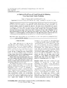
In SPECTF Heart, the accuracy of Clip3 and Clip4 is 77% and the accuracy of 1-NN is 72.1% (Kim and Zhang, 2007; Wang et al., 2005), the accuracy of BPN by using PCA is 75.1%, SBPN is 79% and BPN by using WLA has higher accuracy of others that is 94%. In SPECT Heart, the accuracy of Clip3 is 84% and Clip4 is 90.4% and the accuracy of 1-NN is 80.2%, (Kim and Zhang, 2007; Wang et al., 2005). The accuracy of BPN by using PCA is 73.3%, SBPN is 87% and BPN by using WLA has higher accuracy of others that is 92%. Figures 7 and Figure 8 show the charts of comparison accuracy of classification methods on SPECTF Heart and SPECT Heart datasets. Figure 7: Comparison of classification accuracy on SPECTF Heart dataset 100% 90% 80% 70% 60% 50% 40% 30% 20% 10% 0%
Accuracy
New SMFFNN by using WLA
SBPN
BPN by using PCA
K-NN (K=1)
Clip3
Clip4
94%
79%
75.10%
72.10%
77%
77%
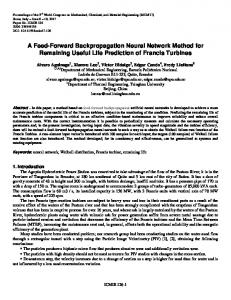
Figure 8: Comparison of classification accuracy on SPECT Heart dataset 100% 90% 80% 70% 60% 50% 40% 30% 20% 10% 0% Accuracy
New SMFFNN by using WLA
SBPN
BPN by using PCA
K-NN (K=1)
Clip3
Clip4
92%
87%
73.30%
80.20%
84%
90%
The accuracy of performance of new SMFFNN by using WLA is better than other methods because it uses real potential weights, thresholds and does not work on random initialization. Comparison on speed of training process of the methods on SPECTF Heart and SPECT Heart dataset is shown in Table 5 as follow: Table 5:
Comparison of classification speed on SPECTF Heart dataset and SPECT Heart Method
Epoch
New SMFFNN using WLA SBPN BPN by using PCA
1 25 14
SPECTF Heart CPU time Error 0.061 0.11 4.98 0.21 1.6 0.25
SPECT Heart CPU time Error 0.036 0.13 2.92 0.15 1.08 0.27
SBPN method performs on SPECTF Heart training dataset in 25 epochs with 4.98 second CPU times and 0.21 error. BPN by using PCA performs on SPECTF Heart training dataset in 14 epochs
175
Roya Asadi, Norwati Mustapha, Nasir Sulaiman and Nematollaah Shiri
with 1.6 second CPU times and 0.25 error. New SMFFNN by using WLA in one epoch during 0.061 second with 0.11 error processes on SPECTF Heart training dataset that has higher speed than other methods. SBPN method performs on SPECT Heart training dataset in 25 epochs with 2.92 second CPU times and 0.15 error. BPN by using PCA performs on SPECT Heart training dataset in 14 epochs with 1.08 second CPU times and 0.27 error. New SMFFNN by using WLA in one epoch during 0.036 second with 0.13 error processes on SPECTF Heart training dataset that has higher speed to other methods. Speed comparison of models and techniques on SPECTF Heart and SPECT Heart datasets are shown in Figures 9 and Figure 10. Figure 9: Comparison of classification speed of BPN and new SMFFNN by using preprocessing techniques on SPECTF Heart dataset
Figure 10: Comparison of classification speed of BPN and new SMFFNN by using preprocessing techniques on SPECT Heart dataset
New Supervised Multi Layer Feed Forward Neural Network Model to Accelerate Classification with High Accuracy
176
New SMFFNN by using WLA preprocessing is faster than other thecniques because training process is in one epoch without training cycle, computing mean square error rate and updating weights. The time complexity of WLA is linear O(pn).
6. Summary and Concluding Remarks Based on the hypothesis of research, new SMFFNN model can get the best result in speed and accuracy by using new preprocessing technique without gradient of mean square error function and updating weights in one epoch. During experiments, the new model was implemented and analyzed using Weights Linear Analysis (WLA). The combination of data pre-processing and new pre-training techniques shows that WLA generated normalized input values and potential weights. This shows that WLA serves as global mean and vectors torque formula to solve the problem. Two kinds of datasets from UCI Repository of Machine Learning are chosen to illustrate the strength of WLA techniques. SPECTF Heart is a multivariate integer dataset and SPECT Heart is a multivariate categorical-binary dataset. The results of BPN by using pre-processing techniques and new SMFFNN with application of WLA showed significant improvement in speed and accuracy. Therefore, the new model with the proposed technique can solve the main problem of finding the suitable weights. The accuracies implementation on two datasets of SPECTF and SPECT Heart are computed by F-measure formula. The results show that robust and flexibility properties of new technique and new SMFFNN model for classification. For future work, we will apply WLA technique into other SMNN model to produce new ones.
References [1] [2] [3] [4] [5] [6] [7] [8] [9]
[10]
Andonie, R. and Kovalerchuk, B. 2004. Neural Networks for Data Mining: Constrains and Open Problems. Computer Science Department Central Washington University, Ellensburg, USA. Cios, K. J., Wedding, D. K. and Liu N. 1997. CLIP3: Cover learning using integer programming, Kybernetes 26 (4–5) (1997) 513–536. Cios, K.J. and Liu, N. 1995. An Algorithm which Learns Multiple Covers via Integer Linear Programming. Part I––The CLILP2 Algorithm, Kybernetes, 24:2, pp. 29–50 (The Norbert Wiener Outstanding Paper Award). Daffertshofer, A., Lamoth, C.J., Meijer, O.G. and Beek P.J. 2004. PCA in studying coordination and variability: a tutorial. Clin Biomech (Bristol, Avon).19:415-428. Dasarathy, B.V. 1991. Nearest neighbor (NN) norms: NN pattern classification techniques. IEEE Comput. Soc. Press, Los Alamitos, CA. DeMers, D. and Cottrell, G. 1993. Non-linear dimensionality reduction. In Advances in Neural Information Processing Systems, volume 5, pages 580–587, San Mateo, CA, USA. Morgan Kaufmann. Demuth, H., Beale, M. and Hagan, M. 2007. Neural Network Toolbox User’s GuideMatlab, The Mathworks, Accelerating the pace of engineering and science. Drago, G.P. and Ridella, S. 1992. Statistically Controlled Activation Weight initialization (SCAWI). IEEE Transactions. on Neural Networks, vol. 3, no. 4, pp. 627-631. Fernández-Redondo, M. and Hernández-Espinosa C. 2001. Weight Initialization Methods for Multilayer feed forward. Universidad Jaume I, Campus de Riu Sec, Edificio TI, Departamento de Informática, 12080 Castellón, Spain. ESANN'2001 proceedings - European Symposium on Artificial Neural Networks. Bruges (Belgium), 25-27 April 2001, D-Facto public., ISBN 2930307-01-3, pp. 119-124. Fernandez-Redondo, M. and Hernandez-Espinosa, C. 2000. A comparison among weight initialization methods for multilayer feedforward networks, Proceedings of the IEEE–INNS–
177
[11] [12] [13] [14] [15] [16] [17] [18] [19] [20]
[21] [22] [23] [24]
[25] [26] [27]
Roya Asadi, Norwati Mustapha, Nasir Sulaiman and Nematollaah Shiri ENNS International Joint Conference on Neural Networks, Vol. 4, Como, Italy, 2000, pp. 543– 548. Funahash, K. 1989. On approximate realization of continuous mappings by neural networks, Neural Networks 2. 183–192. Han, J. and Kamber, M. 2001. Data Mining: Concepts and Techniques. Simon Fraser University, Academic Press. Hegland, M. 2003. Data Mining – Challenges, Models, Methods and Algorithms. May 8. Scientific Literature Digital Library, citeseer.ist.psu.edu/context/68861/0. Hinton, G.E. and Salakhutdinov, R.R. 2006. Reducing the Dimensionality of Data with Neural Networks. Materials and Methods. Figs. S1 to S5 Matlab Code. 10.1126/science. 1127647.June.www.sciencemag.org/cgi/content/full/313/5786/504/DC1 Ho-Sub, Y., Chang-Seok, B. and Byung-Woo, M. 1995. Neural networks using modified initial connection strengths by the importance of feature elements. In Proceedings of International Joint Conf. on Systems, Man and Cybernetics, 1: 458-461. Jolliffe, L.T. 1986. Principal Component Analysis. Springer-Verlag, New York. Jolliffe, L.T. 2002. Principal Component Analysis. Springer. 2nd edition. Keeni, K., Nakayama, K. and Shimodaira, H. 1999. A training scheme for pattern classifcation using multi-layer feed-forward neural networks. In Proceedings of 3rd International Conference on Computational Intelligence and Multimedia Applications, New Delhi, India, pp. 307–311. Kim, J.K. and Zhang, B.T. 2007. Evolving Hyper networks for Pattern Classification. In Proceedings of IEEE Congress on Evolutionary Computation. Page(s):1856 – 1862 Digital Object Identifier 10.1109/CEC. Krzysztof J., Cios and Lukasz A.K. 2003. CLIP4: Hybrid inductive machine learning algorithm that generates inequality rules. Department of Computer Science and Engineering, University of Colorado at Denver, Campus Box 109, P.O. Box 173364, Denver, CO 80217-3364, USA. Department of Electrical and Computer Engineering, University of Alberta, Edmonton, AB T6G 2V4, Canada, Department of Computer Science, University of Colorado at Boulder, Boulder, CO 80309, USA. University of Colorado Health Sciences Center, Denver, CO 80262, USA. 4cData, Golden, CO 80401, USA. Received 8 May 2002; accepted 17 March 2003. Lanckriet, G.R.G., Bartlett, P., Cristianini, N., Ghaoui, L. El and Jordan M. I. 2004. Learning the kernel matrix with semidefinite programming. Journal of Machine Learning Research, 5:27–72. LeCun, Y., Bottou, L., Orr, G. and Muller, K. 1998. Efficient Back Prop. In Orr, G. B. and. Muller, K.-R., (Eds.), Neural Networks: Tricks of the trade, (G. Orr and Muller K., eds.). Lindsay, S. 2002. A tutorial on Principal Components Analysis. February 26. Unpublished. T.Z.1-4244-1340-0/07/2007 IEEE URL://http://www.ics.uci.edu/~mlearn/MLRepository.html Mark W. Craven and Jude W. Shavlik, 1997. Using Neural Networks for Data Mining. Computer Science Department, Carnegie Mellon University, University of Wisconsin-Madison. Elsevier Science Publishers B. V. Amsterdam, The Netherlands, The Netherlands. ISSN: 0167739X. Mariyam, S. 2000. Higher Order Centralized Scale-Invariants for Unconstrained Isolated Handwritten Digits. PhD. Thesis, University Putra Malaysia. P.M. Murphy, “Repository of Machine Learning and Domain Theories”, 1997; http://archive.ics.uci.edu/ml/datasets/SPECTF+Heart; http://archive.ics.uci.edu/ml/datasets/SPECT+ Heart. Neal, M.J., Goodacre, R. and Kell, D.B. 1994. The analysis of pyrolysis mass spectra using artificial neural networks. Individual input scaling leads to rapid learning. In Proceedings of the World Congress on Neural Networks. International Neural Network Society San Diego, California, I-318 - I-323.
New Supervised Multi Layer Feed Forward Neural Network Model to Accelerate Classification with High Accuracy [28] [29] [30] [31]
[32] [33]
[34]
178
Russell, I.F. 2007. Neural Networks. Department of Computer Science. University of Hartford West Hartford, CT 06117. Journal of Undergraduate Mathematics and its Applications, Vol 14, No 1. Shlens, J. 2005. A Tutorial on Principal Component Analysis. Unpublished, Version 2. Van der Maaten, L.J.P., Postma, E., and van den Herik, H. 2008. Dimensionality Reduction: A Comparative Review. MICC, Maastricht University, P.O. Box 616, 6200 MD Maastricht, The Netherlands. Preprint submitted to Elsevier, 11 January. Wang, J., Kwok, J.T., Shen, H.C. and Quan, L. 2005. Data-Dependent Kernels for HighDimensional Data Classification. In Proceedings of International Joint Conference on Neural Networks, Montreal, Canada, July 31 - August 4, 2005. 0-7803-9048-2/05/2005 IEEE. Department of Computer Science The Hong Kong University of Science and Technology Clear Water Bay Hong Kong. Werbos, P.J. 1974. PaulWerbos. Beyond Regression: New Tools for Prediction and Analysis in the Behavioral Sciences. PhD thesis, Committee on Applied Mathematics, Harvard University, Cambridge, MA, November 1974. Zhang, X.M., Chen, Y.Q., Ansari, N. and Shi, Y.Q. 2003. Mini-max initialization for function Approximation. Department of Electrical & Computer Engineering, New Jersey Institute of Technology, Newark, NJ 07102, USA. Department of Computer Science and Engineering, Intelligent Information Processing Laboratory, Fudan University, People’s Republic of China. Accepted 31 October 2003. Yim, T.K. 2005. An Improvement on Extended Kalman Filter for Neural Network Training. Master Thesis, University Putra Malaysia.