An Artificial Neuron (ANN) is a model of biological neuron. ..... [7] G. P. J. Schmitz, C. Aldrich, and F. S. Gouws, ANN-DT An Algorithm for Extraction of Decision.
International Journal on Computational Sciences & Applications (IJCSA) Vol.4, No.2, April 2014
Feed Forward Neural Network For Sine Function With Symmetric Table Addition Method Using Labview And Matlab Code Fadhil A. Ali Department of Electrical and Computer Engineering- Oklahoma State University 202 Engineering South Stillwater, OK 74078 USA- Tel:405-714-1084
Abstract This work is proposed the feed forward neural network with symmetric table addition method to design the neuron synapses algorithm of the sine function approximations, and according to the Taylor series expansion. Matlab code and LabVIEW are used to build and create the neural network, which has been designed and trained database set to improve its performance, and gets the best a global convergence with small value of MSE errors and 97.22% accuracy.
Keywords Neural networks, Symmetric Table Addition Method, LabVIEW , Matlab scripts
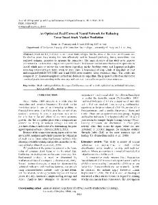
1.Introduction 1.1 Artificial Neural Network An Artificial Neuron (ANN) is a model of biological neuron. Many of ANN receives signals from the environment or other ANNs, and its gathering these signals by using activation function to the signals sum. Input signals are excited through positive or negative numerical weights that associated with each connection to the ANNs, thus firing of the ANN and the strength of the exciting signal are controlled via a function referred to as activation function. The ANNs are collecting all incoming signals and computing a net input signals as a function of the respective weights. The net input renders to the activation function by calculated the output signal of the ANNs, which is called the layered network. ANN may consist of input, hidden and output layers [1], as shown in Figure (1).
Figure (1) Neural Network Architecture
The ANN is designed to work similar to neural tissue in the brain, where many independent neurons (processing units) are interconnected into one large data-processing network. In the ANN DOI:10.5121/ijcsa.2014.4201
01
International Journal on Computational Sciences & Applications (IJCSA) Vol.4, No.2, April 2014
the “neurons” are represented as mathematical functions, which pass the data between themselves in some defined and organized manner. The way of organization of the connections between the “neurons” defines the features of the ANN, and its capability to perform certain tasks [2]. One of the simplest ANN’s is a feed-forward network, which it has worked in this investigation, therefore other types of ANN will not be considered here. Such a network consists of: one input layer, hidden layers (i.e. nodes)-(possibly more than one) and one output layer. The data are transferred in a form of “signals”, it means values which are passed between the nodes. Each connection among the nodes has a special variable associated with it – this is a weight. Each neuron collects all the input values multiplied by the associated weights and processes them with activation function: S
,
=
∑S
,
.W
,
………….. (1)
where: f – Activation function, Sx,i – output signal of ith neuron in xth layer, Sx-1,i – output of ith neuron in x-1th layer, Wx,i – weights connected to neuron Sx,i. The ‘response’ is an activation function output of a given neuron, that is simply named the “neuron function”. The most activation functions are: 1.Sigmoid function :
2.Gaussian function :
( )=
(
………………….. (2)
σ
)
( ) = exp (− )…………………. (3) σ
Definitely, any neural network is training a number of times that will give the results in a stronger weight of neurons but could not exceed the specific limits. This can be causes the network to memorize instead of learning [3]. 1.2 Symmetric Table Additional Method Symmetric Table Addition Methods (STAMs) use two or more parallel table lookups followed by multi operand addition to approximate the elementary functions. These methods stake advantage of symmetry and leading sign bits in the table entries to drastically reduce the size of the table. In [5] the method produces tables for the symmetric table addition method for approximating a function f(x). The inputs n0, n1, n2, and n3, which corresponds to the number of bits in x0, x1, and x2 are taken by STAM , where x = x0 + x1 + x2 + x3. It also takes as input the number of guard digits," ng ", and a variable " f" , which indicates the function to be implement. This procedure computes the coefficients produced by this approximation method, and reports on the maximum and average error of the approximations. According to Nihal Koc-Sahan et al[6], the multi-layer perceptron networks, the inputs to the sigmoid function and its derivate correspond to sums of weighted values. And x typically has the form; x=bm-1bm-2….b0b-1b-2…b-p ………….(4) Where x is n-bit fixed point number. 2
International Journal on Computational Sciences & Applications (IJCSA) Vol.4, No.2, April 2014
Then STAMs divide the input operand, x, into m+1 bit partitions, x0,x1,…xm. This approximation is based on two term Taylor series expansion.
1.3 Decision Tree The decision tree (DT) is an algorithm tool that uses a tree-like graph or model for taken decisions and their possible consequences, including chance event outcomes. The DTs are commonly used in operations research and decision analysis, to help identification strategy of the most likely to reach a goal. This goal is to create a model that predicts the value of a target variable based on several input variables. The tree also can be "learned" by splitting the source set into sub-sets based on an attribute value tests. This process is repeated on each derived sub-set in a recursive manner , which is recursive partitioning. The recursion process is completed when the sub-set at a node for all that has the same value of the target variable, or when splitting no longer adds value to the predictions. In data mining, many trees algorithms can be described as the combination of mathematical and computational techniques to aid the description, categorization and generalization of a given set of data. Data refers in the specific records of the form: (x, Y)=(x 1, x 2, x 3… x k, Y) ……................…. (5) Y is the dependent variable, which is the target variable that must be understand and classify. Also, a vector x is composed of the input variables ( x1, x2, x3...xk ), those are used for such task of calculations [7, and 8].
2.Proposed method In traditional neural network with sigmoid activation function has the advantage, it can approximate any continuous function but gets the fail in ending up as large network as possible. The goal in this paper is to design a neuron synapse of multi-layer network. The proposed method uses sine function as building blocks, and combine together by adapting STAMs parameters to build a final function. This has achieve a fitting performance for the training data of the present network, and it has taking a tree formulation (DT) which the function was modeled. Since that many literatures have proposed and used tree form of neural networks [9, 10, and 11]. In computer algebra and symbolic computations a function can be represented as tree representation [12]. Its tree form of sine function and operation gets our neural network of trained data to build the node. The node represents a sine function applied to the sum of STAM’s parameters, and each terminal node represents input variables and gets its child nodes. By using Taylor series expansion of sine function E ( ); E( )=
−
!
+
!
−
!
+ ⋯,
= 0 …….....…...........………. (6)
Where is the input argument and Let us construct the tree
are parameters (weights) in our network.
Y=E( 2+ E ( 1)) + E ( 2) .......………. (7) 3
International Journal on Computational Sciences & Applications (IJCSA) Vol.4, No.2, April 2014
The training data set has taken an incremental way to perform new data set. The algorithm is used the following steps for getting a forward network [13]; 1- Start from a blank network. Initialize all weights to zero. 2- Testing the effect of adding a layer to the network performance, as follows: a- Set up the current network configuration. b- Add a layer to the current network by selecting the layer and terminating node types. c- The nodes weights for the existing network are initialized by STAM’s values, d- The optimization algorithm is applied to the new network scheme and find out the resulting network performance accordingly. e- Keeping the new added layer. f- Repeat step 2 to get all possible sine function Taylor series terms. The database is selected as randomized values during the test interval, in order to make sure that the network learns instead of memorize. Insufficient training may lead to incorrect results. Thus, training must be done until 100% training accuracy is achieved. Figure (2) shows the flowchart for training and testing the database.
. Figure (2) Flowchart of the training and testing data
On Taylor series, there are expansions for sin function, which are given in terms of odd powers of x, in this work 6 input nodes have been taken with x,x3,x5,x7,x9, and x11. Therefore, all the powers of x with alternating zero weights; (Sin: 0, 1, 0, -1/6...,). Therefore, the built up neural network has got each input to one corresponding node, and multiplied it by its weight to fed entire possible outputs to the output nodes, it would be capable of the 6-terms Taylor's expansion of a sine function. 4
International Journal on Computational Sciences & Applications (IJCSA) Vol.4, No.2, April 2014
Inputs
Hidden layer
Outputs
x1 --------------- H0 --------------------/// x3 --------------- H1 --------------------/// x5 --------------- H2 --------------------/// x7 --------------- H3 --------------------/// x9 --------------- H4 --------------------/// x11 --------------- H5 --------------------/// Figure (3) explicit representation of the presented neural network
3 .Symmetric table additional method (STAM) - Neuron The conventional neural network shown in Figure (3) has shown the single variable weight i is replaced by STAM block diagram shown in Figure (4) [6], which a multi operand adder has cancelled to get a STAM neuron been established and it is shown in Figure(5).
Figure (3) a conventional neural network
5
International Journal on Computational Sciences & Applications (IJCSA) Vol.4, No.2, April 2014 Figure (4) STAM block diagram
Figure (5) STAM‘s Neuron
4.LabVIEW Design In this section, the system architecture is described in LabVIEW block diagram. It has four processing stages as seen in Figure (6).The system is initialized when a data collected from datasheets, followed with neural network configuration, draw the network , resize the inputs and finally initiate nodes. LABVIEW is used as a design platform for the system that is illustrated in flowchart steps.
Figure (6) NN LabVIEW System’s flowchart
The processing of collected data includes inputs and operands of STAM output. This work focuses on application of STAM algorithm gets the design of neuron synapses of the Neural Network for a sine function which is the third stage of the designed system.
6
International Journal on Computational Sciences & Applications (IJCSA) Vol.4, No.2, April 2014
A database was created to accomplish Neural Network System (NN system) comprising data used for experimental purpose. The database is pre-trained and tested using Matlab script function[14], which is integrated with LabVIEW for real- time testing.
5.Results & Discussion This section detaches the parameter setting for the neural network architecture system. In addition to that, the (training, testing and real- time) data resulted are also discussed in some details.
5.1 Parameters Setting After many attempts, it was found that the following parameters yield around 100% of training accuracy. The error measure used to assess the network performance is Mean Square Error (MSE) as follows [13]; MSE =
( )
( )
……...............................................................(8)
where y (j), d (j) are the network output and the desired output j respectively, and J is the size of the data set. Most of error measures and the number of weights in the resulted network, which is given to compare the network complexities. Table (1) shows the most parameters used with the training results. Table (1) Details of Training and Testing for ANN
Feed forward neural network algorithm Defined Parameters Transferred function Tan sig Number of Hidden Neurons 6 Set the Performance Goal 1e-10 The Momentum Factor 0.9 The Learning Rate 0.01 The Total number of terms in the Taylor series (sine function): 200 Training and Testing Parameters The Training Epoch 50 The Training Time 0:00:01 The Training Accuracy 100% The Testing Accuracy 97.22% The data training has been conducted, and tan-sig is chosen as a transfer function for the layers as it converges. Also, the number of hidden neurons has been set to 6 neurons. The Learning rate and performance goal is set to a lower value , so that the network learns completely. A momentum factor of 0.9 is added in the network which can be recover back for training even if it falls into local minimum. 5.2 Training Results In figure (7), 100% training accuracy met with 50 iterations. It shows the neural network toolbox illustrating the transfer function, iterations and performance goal that is achieved during training. The amount of 100 terms out of 112 inputs are 89% of the data were successfully trained as seen 7
International Journal on Computational Sciences & Applications (IJCSA) Vol.4, No.2, April 2014
in the performance and regression plots in figure (8) and figure (9), with 100% training accuracy respectively. Regression plot has shown the data are fitted the line when the training is complete. Also, training state is shown in figure (10) indicates the closer in the accuracy percentage.
Figure (7) NN system toolbox
Figure (8) NN system performance
8
International Journal on Computational Sciences & Applications (IJCSA) Vol.4, No.2, April 2014
Figure (9) NN system regression plots
Figure (10) NN system training state plots
5.3 Testing Results All the terms in the database which is 112 were used for testing purpose. The data was randomized before testing so that the system has an accurate performance for sine function (Target). The testing accuracy that has been achieved is 97.22% for 112 inputs of the system. According to this result, that achieved a higher rates, figure (11) is shown the sine function in both exact and predicted by the present NN system, while figure (12) illustrates the fitting curves of the resulted sine function.
9
International Journal on Computational Sciences & Applications (IJCSA) Vol.4, No.2, April 2014
Figure (11) sine function plots
Figure (12) Fitting of sine function plot
5.4 Real-Time Testing Real- time testing has been done for the complete system. The trained network was integrated in LABVIEW. A GUI panel was designed in LABVIEW indicating the neural network graph in database as set in Table (1). Random numbers is generated if targeted function data was found not to be in database. This can be seen from figures (13, and 14) respectively, the frontal system was designed in LABVIEW for a real- time application with a high accuracy.
10
International Journal on Computational Sciences & Applications (IJCSA) Vol.4, No.2, April 2014 Figure (13) configuration frontal of NN system
Figure (14) NN system training frontal
6 .Conclusion This paper gives a proposed method to create symmetric table additional method (STAM) neuron. Which it represented the general aspects of a sine function behavior and indicates the neuron synapses in neural network design for a real-time application used and designed in LABVIEW integrating the Neural Network from MATLAB codes embedded in the system. A minimized MSE rate to give the presented value 97.22% has been achieved of the neural network accuracy.
7.Acknowledgement Many thanks to Oklahoma State University and – School of Electrical and Computer Engineering Department for hosting me as visitor scholar. My deep appreciation to Dr. James E. Stine for his valuable notes. Also, many thanks to SRF/IIE for giving me all possible supports.
References [1] [2] [3]
[4] [5]
[6]
Andries P. Engelbrecht, Computational Intelligence: An Introduction - second edition, John Wiley & Sons Ltd, 2007 D.T. Pham, X. Liu, Neural networks for identification, prediction and control, Springer-Verlag London Ltd. UK, 1995 N. F. Naim, A. I. M. Zakaria, N. A. Wahab, Classification of Thumbprint using Artificial Neural Network (ANN), IEEE International Conference on System Engineering and Technology (ICSET), Shah Alam, 2011, pp. 231- 234 A. Reda, B. Aoued, Artificial Neural Network Based Face Recognition, First International Symposium on Control, Communications and Signal Processing, Algeria, 2004, pp. 439- 442 J.E.Stine and M.J.Schulte, The Symmetric Table Addition Method for Accurate Function Approximation, Journal of VLSI Signal Processing Systems for Signal, Image, and Video Technology, vol.21,1999,pp.167-177 Nihal Koc-sahan , Jason A. Schlessman , Michael J. Schulte, Symmetric table addition methods for neural network approximations,Proc. SPIE 4474, Advanced Signal Processing Algorithms, Architectures, and Implementations XI, 2001,pp.126-133
11
International Journal on Computational Sciences & Applications (IJCSA) Vol.4, No.2, April 2014 G. P. J. Schmitz, C. Aldrich, and F. S. Gouws, ANN-DT An Algorithm for Extraction of Decision Trees from artificial Neural Networks, IEEE Transactions on Neural Networks,vol.10,No.6,1999,pp.1392-1401 [8] I. K. Sethi, Layered Neural Net Design Through Decision Trees, IEEE International Symposium on Circuits and Systems, vol.2,1990,pp.1082-1085 [9] S. Behnke, and N. B. Karayiannis, Competitive neural trees for pattern classifications IEEE Transactions on Neural Networks,vol.9,No.6,1998,pp.1352–1369 [10] A. Sankar, and R. J. Mammone, Growing and pruning neural tree networks, IEEE Transactions on Computers,vol.42,No.3,1993, pp.291–299 [11] B.T. Zhang, A Bayesian evolutionary approach to the design and learning of heterogeneous neural trees, Integrated Computer- Aided Engineering,vol.9,2002,pp.73–86 [12] J. S. Cohen, Computer algebra and symbolic computation: Elementary algorithms. Natick: A. K. Peters, Ltd,2002 [13] George S. Eskander and Amir F. Atiya, neural networks, Neural Networks ,vol.22 ,2009,pp. 395–404 [14] Forrester W. Isen , DSP for MATLAB and LabVIEW: Fundamentals of Discrete Signal Processing, Morgan & Claypool publishers ,2009 [7]
12