Oct 10, 2006 - [7] Raskar R., Ilie A., Yu J.: Image Fusion for Context Enhancement and Video Surrealism. Proceedings of the Third International Symposium on ...
Nonlinear Multiresolution Image Blending Mark Grundland, Rahul Vohra, Gareth P. Williams and Neil A. Dodgson Computer Laboratory, University of Cambridge, United Kingdom
October 10, 2006 Abstract. We study contrast enhancement for multiresolution image blending. In image compositing, image stitching, and image fusion, a blending operator combines coefficients of a pixel array, an image pyramid, a wavelet decomposition, or a gradient domain representation. Linear interpolation reduces variation and thereby causes contrast loss, while coefficient selection increases variation and thereby causes color distortion. Offering a continuous range of possibilities between these standard alternatives, the signed weighted power mean enables the user to calibrate the contrast of composite images. Key words: Multiresolution contrast enhancement, image compositing, image blending, image fusion, image stitching, image pyramid, image editing, video editing, cross dissolve, digital art.
1. Introduction We1 demonstrate a new way to enhance contrast during multiresolution image blending. The task of image blending techniques is to produce a coherent composite image from a weighted combination of component images. In image and video editing, image blending is utilized for image compositing [3, 8], image stitching [1, 2, 6] and image fusion [4, 5, 7]. Standard image blending [3] linearly combines pixel values using a weighted average. It is well known to cause double exposure in image compositing, visible seams in image stitching and detail loss in image fusion. To address these problems, image blending can be performed on various image representations, including multiresolution image pyramids [1, 2, 4, 8], wavelet decompositions [5], and gradient domain representations [6, 7]. The coefficients of multiresolution image representations must be combined with care to prevent artifacts. As recently surveyed [5], the two most common multiresolution image blending operators are linear interpolation [1] and coefficient selection [2]. Linear interpolation outputs a weighted sum of the coefficient values. As an averaging operation, it reduces variation. The resulting contrast loss and color fading can diminish the visibility of image details (Figure 1b). Coefficient selection outputs the coefficient value with the maximal absolute magnitude. As a discontinuous operation, it increases variation. The resulting contrast gain and color aberrations can amplify the appearance of image distortions (Figure 1e). When combining coefficients of similar magnitude but opposite sign, linear interpolation causes cancellation while coefficient selection causes instability. 1 Send correspondence to Mark Grundland: Mark @ eyemaginary.com A color version of this paper is available: http://www.eyemaginary.com/Portfolio/Publications.html
Machine GRAPHICS & VISION vol. , no. , pp.
2
Nonlinear Multiresolution Image Blending
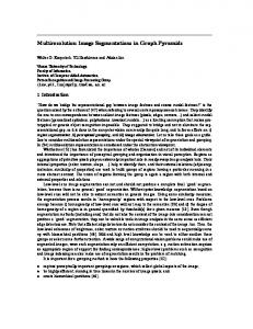
Lake: 40% opacity
Horizon: 20% opacity
Couple: 40% opacity
(a) Contrast de-enhancement U = 0.5
(b) Linear interpolation [1,3] U = 1.0
(c) Weak contrast enhancement U = 2.0
(d) Strong contrast enhancement U = 4.0
(e) Coefficient selection [2] U=
(f) Contrast preservation [8]
(a) U = 0.5
(b) U = 1.0
(c) U = 2.0
(d) U = 4.0
(e) U =
(f)
Fig. 1. When performing multiresolution image blending using Laplacian pyramids, our contrast enhancement technique enables users to find an appropriate balance (c)-(d) between contrast reduction (a)-(b) and color distortion (e)-(f) by specifying the parameter value ρ of our nonlinear operator.
Machine GRAPHICS & VISION vol. , no. , pp.
Mark Grundland, Rahul Vohra, Gareth P. Williams and Neil A. Dodgson
3
As these opposing strategies can have undesirable consequences, users seek a balance between them. Our novel nonlinear image blending operator, the signed weighted power mean, generates the intermediate renditions (Figure 1a-e) between linear interpolation and coefficient selection. It offers a flexible method for calibrating contrast in composite images. Unlike previous pattern selective operators [4], it supports user specified opacity maps to weigh the components’ contributions to the composite. As a separate and complementary approach, it can be readily integrated with our techniques [8] for preserving contrast, color, and salience in image compositing. For comparison, we demonstrate the result of multiresolution contrast preserving compositing (Figure 1f), which recovers the contrast lost due to linear interpolation by linearly transforming composite coefficients. 2. Method Given n component images with corresponding coefficients ak ∈ R and opacity maps � wk = 1, we define (Figure 2) their wk ∈ [0, 1], specifying nonnegative convex weights signed weighted power mean C using the signed power function Tρ (a): � � n � ρ wk Tρ (ak ) for Tρ (a) = sign(a) |a| (1) C = T ρ1 k=1
This image blending operator allows users to fine-tune contrast enhancement along a continuous spectrum 0 < ρ < ∞ of possibilities. Observe that the combined coefficient C respects the range of its component coefficients, min ak ≤ C ≤ max ak . When ρ = 1, we � obtain linear interpolation [1], where C = wk ak , which reduces contrast (Figure 1b). When ρ → ∞, we obtain coefficient selection [2], where C = arg max |ak |, which maximizes contrast (Figure 1e). When ρ = 2, we obtain a signed quadratic average which raises contrast by a reasonable amount (Figure 1c). For a more pronounced contrast enhancement effect (Figure 1d), we suggest ρ = 4 . For a contrast de-enhancement effect (Figure 1a), we suggest ρ = 12 . Finally, if ρ → 0, contrast is minimized by taking a signed geometric average of the coefficients when they all share the same sign and taking zero otherwise. For pattern selective blending [4], the exponent ρ can locally depend on the content of the component images. A low exponent can be used to merge similar regions while a high exponent can be used to select between divergent regions. We apply our image blending operator using Laplacian image pyramids [1, 2]. They serve to decompose the images into successive levels of detail, enabling image blending to be performed at each level independently. In effect, only image features of comparable scales are directly combined with each other. Allowing low frequency image structures to be blended over larger regions than high frequency image details serves to improve the visual coherence of the composite. We represent the component images’ RGB color channels by Laplacian pyramids and their opacity maps by Gaussian pyramids. Starting Machine GRAPHICS & VISION vol. , no. , pp.
4
Nonlinear Multiresolution Image Blending
1 0.5 0 -0.5 -1 -1 1
1 0.5 0
1 0.5 0 -0.5 -1 -1 1
-0.5
1 0.5 0 -0.5
-0.5
0
U = 0.50
0.5
U = 0.75
1 -1
1 0.5 0 -0.5 -1 -1 1
1 0.5 0
1 -1
1 0.5 0 -0.5 -1 -1 1
-0.5
1 0.5 0 -0.5
-0.5
0
U = 1.00
0.5
U = 2.00
1 -1
1 0.5 0 -0.5 -1 -1 1
1 0.5 0 -0.5
1 -1
1 0.5 0 -0.5 -1 -1 1
1 0.5 0 -0.5
-0.5
0
-0.5
0
0.5
Fig. 2.
-0.5
0
0.5
U = 4.00
-0.5
0
0.5
0.5 1 -1
U=
The signed power mean with equal weights w1 = w2 =
1 -1 1 2
and varying parameter values ρ.
Machine GRAPHICS & VISION vol. , no. , pp.
5
Mark Grundland, Rahul Vohra, Gareth P. Williams and Neil A. Dodgson
City by night [7]
City by day [7]
Opacity mask [7]
(a) Linear interpolation using pixel colors [3]
(b) Specialized image fusion using the gradient domain [7]
(c) Linear interpolation using Laplacian pyramids [1]
(d) Signed weighted power mean using Laplacian pyramids
(e) Coefficient selection using Laplacian pyramids [2]
(f) Contrast preserving blending using Laplacian pyramids [8]
(a) [3] Fig. 3.
(b) [7]
(c) [1]
(d) New
(e) [2]
(f) [8]
Our nonlinear image blending operator reduces fading, discoloration, and halo artifacts.
Machine GRAPHICS & VISION vol. , no. , pp.
6
Nonlinear Multiresolution Image Blending
with the image at the base, each level of a Gaussian lowpass pyramid is constructed by filtering the previous level with a binomial filter and subsampling the result. A Laplacian bandpass pyramid stores the differences between successive levels of a Gaussian pyramid. To allow reconstruction, the top level of the Gaussian pyramid is retained atop the Laplacian pyramid. For image blending, the corresponding coefficients of each level of the Laplacian pyramids are combined according to the weights specified in their Gaussian pyramids. We apply the signed weighted power mean to combine the corresponding bandpass coefficients and the normal linear weighted average to combine the corresponding top level lowpass coefficients. For ρ = 1 and spatially constant opacities (Figure 1b), linear cross dissolve using Laplacian pyramids [1] is equivalent to linear interpolation of pixel values [3] since the Laplacian pyramids are constructed using linear filtering. 3. Applications As a case study, we experimented with image fusion of a scene captured during the day and at night [7]. In this visualization application (Figure 3), the daytime picture provides contextual information for the interpretation of the nighttime activities. Derived from an additional clean plate image [7], an opacity map determines the relative contribution of each component. For image fusion, a robust image blending technique should be able to cope with minor inaccuracies in such opacity maps. We compared a range of algorithms exhibiting different kinds of artifacts (observe the windows of the building on the right). Linear averaging of pixel values [3] is not effective as it generates too abrupt transitions between day and night (Figure 3a). The blending algorithm [7] originally designed for this task, which operates in the gradient domain [6], produces a faded rendition with a slight blur (Figure 3b). The remaining methods rely on Laplacian image pyramids. Linear interpolation [1], with ρ = 1, suffers from reduced contrast as well as halo artifacts (Figure 3c). Contrast preserving blending [8] offers more contrast but still has some halo artifacts (Figure 3f). These halo artifacts reflect the smoothing properties of the multiresolution image pyramid. On the other hand, coefficient selection [2], with ρ → ∞, produces sharp contrast as well as severe color distortion (Figure 3e). These color artifacts are due to separate processing of correlated color channels, where one color channel receives the daytime data while another color channel receives the corresponding nighttime data. Our nonlinear image blending operator, the signed weighted power mean with ρ = 4, steers the middle ground, offering good contrast with just a hint of a color halo (Figure 3d). Unlike most other image blending methods [1, 2, 3, 6], we enable the user to ultimately decide what level of contrast enhancement is appropriate. We also used nonlinear blending to render a cross dissolve visual transition (Figure 4) and we measured its contrast (Figure 5). For high ρ values, the brightest and darkest regions of the images take longer to fade out, as their contributions dominate the signed weighted power mean. Contrast preserving blending [8] does not exhibit this behavior. Machine GRAPHICS & VISION vol. , no. , pp.
7
Contrast preservation
ȡ=
ȡ = 4.0
ȡ = 2.0
ȡ = 1.0
ȡ = 0.5
Mark Grundland, Rahul Vohra, Gareth P. Williams and Neil A. Dodgson
Į = 0.1
Į = 0.2
Į = 0.3
Į = 0.4
Į = 0.5
Į = 0.6
Į = 0.7
Į = 0.8
Į = 0.9
Fig. 4. A nonlinear cross dissolve is produced by varying the opacity α so that w1 = α and w2 = 1 − α.
4. Conclusion This work extends our earlier research [8] into creating composite images which preserve the contrast, color and salience of their components. In this work, we propose a simple, efficient, and continuous, nonlinear operator designed for multiresolution image blending, providing users with flexible, high-level control over the appearance of composite imagery. Machine GRAPHICS & VISION vol. , no. , pp.
8
Nonlinear Multiresolution Image Blending
Dissolve Contrast visual Levels transition Contrast of Cross a cross dissolve
Contrast level: average standard deviation Contrast Level of the RGB color channels
0.32
0.3
ȡ=
0.28
ȡ = 4.0 0.26
Contrast preservation
0.24
ȡ = 2.0 0.22
0.2
ȡ = 1.0
0.18
ȡ == 0.5 rho 0.5 ȡ == 11.0 rho ȡ == 22.0 rho ȡ == 44.0 rho ȡ == infinity rho PreservePreserving contrast Contrast
0.16
ȡ = 0.5 0
0.1
0.2
0.3
0.4
0.5
0.6
0.7
0.8
0.9
1
Alpha Opacity factor: Į
Fig. 5. For ρ = 4, our nonlinear image blending operator maintains steady contrast during cross dissolve.
References 1983 [1] Burt P.J., Adelson E.H.: A Multiresolution Spline with Application to Image Mosaics. ACM Transactions on Graphics, 2(4), 217-236. 1984 [2] Burt P.J.: The Pyramid as Structure for Efficient Computation. Multiresolution Image Processing and Analysis, Springer-Verlag, 6-35. [3] Porter T., Duff, T.: Compositing Digital Images. Proceedings of SIGGRAPH, 253-259. 1993 [4] Burt P. J., Kolczynski R.J.: Enhanced Image Capture through Fusion. Proceedings of the International Conference on Computer Vision, 173-182. 1999 [5] Zhong Z., Blum R.S.: A Categorization of Multiscale-Decomposition-Based Image Fusion Schemes with a Performance Study for a Digital Camera Application. Proceedings of the IEEE, 87(8), 13151326. 2003 [6] Perez P., Gangnet M., Blake A.: Poisson Image Editing. Proceedings of SIGGRAPH, ACM Transactions on Graphics, 22(3), 313-318. 2004 [7] Raskar R., Ilie A., Yu J.: Image Fusion for Context Enhancement and Video Surrealism. Proceedings of the Third International Symposium on Non-photorealistic Animation and Rendering, 85-94. 2006 [8] Grundland M., Vohra R., Williams G.P., Dodgson N.A.: Cross Dissolve without Cross Fade: Preserving Contrast, Color and Salience in Image Compositing. Proceedings of EUROGRAPHICS, Computer Graphics Forum, 25(3), 577-586.
Machine GRAPHICS & VISION vol. , no. , pp.
9
Mark Grundland, Rahul Vohra, Gareth P. Williams and Neil A. Dodgson
Church
Opacity map
Forest
(a) Contrast de-enhancement U = 0.5
(b) Linear interpolation [1] U = 1.0
(c) Weak contrast enhancement U = 2.0
(d) Strong contrast enhancement U = 4.0
(e) Coefficient selection [2] U=
(f) Contrast preservation [8]
(a) U = 0.5 Fig. 6.
(b) U = 1.0
(c) U = 2.0
(d) U = 4.0
(e) U =
(f)
Our nonlinear image blending operator is applied using a linear gradient as an opacity map.
Machine GRAPHICS & VISION vol. , no. , pp.
10
Nonlinear Multiresolution Image Blending
Lake
Opacity map
Couple
(a) Contrast de-enhancement U = 0.5
(b) Linear interpolation [1] U = 1.0
(c) Weak contrast enhancement U = 2.0
(d) Strong contrast enhancement U = 4.0
(e) Coefficient selection [2] U=
(f) Contrast preservation [8]
(a) U = 0.5 Fig. 7.
(b) U = 1.0
(c) U = 2.0
(d) U = 4.0
(e) U =
(f)
Our nonlinear image blending operator is applied using a radial gradient as an opacity map.
Machine GRAPHICS & VISION vol. , no. , pp.