European Congress on Computational Methods in Applied Sciences and Engineering ECCOMAS 2000 Barcelona, 11-14 September 2000 ECCOMAS
NUMERICAL ESTIMATION OF FRACTURE PARAMETERS IN ELASTIC AND ELASTIC-PLASTIC ANALYSIS T. Denyse de Araújo*, T.N. Bittencourt†, D. Roehl*, and L.F. Martha* *
Departamento de Engenharia Civil Pontifícia Universidade Católica do Rio de Janeiro (PUC-Rio) Rio de Janeiro, RJ, 22453-900, Brazil E-mail: {denyse,droehl,lfm}@civ.puc-rio.br †
Departamento de Estruturas e Fundações e Laboratório de Mecânica Computacional Universidade de São Paulo (EPUSP) São Paulo, SP, 05508-900, Brazil Email:
[email protected]
Key words: Finite Elements, Fracture Mechanics, Elastic-Plastic Analysis. Abstract. The finite element method has been largely used to analyze mechanical problems and, in particular, to obtain the response of cracked structures. One of the major issues in using the method is mesh generation. Nowadays, several automatic mesh generation algorithms are available for two-dimensional models. Crack analysis imposes severe requirements on automatic mesh generation. It is not uncommon that elements near the cracktip be two orders of magnitude smaller than other elements in the model. Meshing algorithms must be able to provide good size transition capabilities. Previous works of the authors have proposed techniques for automatic, self-adaptive mesh generation of two-dimensional cracked models1. This work describes the numerical procedures that were developed to numerically estimate fracture parameters both in linear-elastic and elastic-plastic analysis. The article describes three methods to evaluate fracture parameters: Displacement Correlation Technique2, Modified Crack Closure Method3, and J-integral evaluation accomplished by means of Equivalent Domain Integrals4. The latter method is also used to evaluate fracture parameters in elastic-plastic analysis. In the mesh generation procedure, special elements with well-formed shape are placed at the crack-tips. For linear-elastic analysis, quarter-point triangular elements are used, forming a rosette of elements with angles of 45°, 40°, or 30°. In elastic-plastic analysis, collapsed Q8 elements are used in the standard rosette. The von Mises yield criterion, with isotropic hardening, is used in the plastic analysis. Some examples are presented to compare the results with analytical and other available numerical results.
1
T. Denyse de Araújo, T.N. Bittencourt, D. Roehl, and L.F. Martha.
1
INTRODUCTION
The finite element method has been widely employed for the solution problems in linear elastic and elastic-plastic fracture problems. However, the high stress and strain gradients near the crack tip require very refined meshes and special elements at the crack tip. An interactive graphics computational system5 is used to introduce the crack in the model and to generate the mesh. Mesh generation is based on recursive spatial enumeration techniques: a binary tree partition for the boundary and the crack-line curves refinement and a quadtree partition for domain mesh generation. In this scheme, the advantages of the algorithm based on quadtree properties are combined with the advantages of a boundary contraction triangulation technique, which is based on Delaunay properties. To generate finite elements, templates are applied to quadtree cells in the entire domain, except in the narrow region close to the boundary, where the boundary contraction triangulation is used. To insure well-shaped elements at crack tips, uniform rosettes of elements are used around each tip. The standard rosette is formed by eight elements, each one with an angle of 45°, usually aligned with the crack-line (Figure 1a). Conventional triangular elements (T6), quarter-point singular elements6, or the collapsed Q8 elements7 can compose the rosette. In this work, five types of rosettes were implemented, distinguished by the element types and angles. They are: a) T6 non singular elements in the standard rosette (Figure 1a); b) Collapsed Q8 elements in the standard rosette (Figure 1a); c) Quarter-point singular elements in the standard rosette (QP45 - Figure 1a); d) Quarter-point singular elements in a rosette with an angle of 40° (QP40 Figure 1b); e) Quarter-point singular elements in a rosette with an angle of 30° (QP30 Figure 1c).
Figure 1: Rosettes of finite elements. (a) Standard rosette (T6, QP, Q8C); (b) Rosette with QP elements to 40o; (c) Rosette with QP elements to 30o.
The main objective of this work is a comparison of the results obtained with the five types of rosettes and an evaluation of several methods that compute numerically the fracture parameters. The quarter-point triangular elements, rosettes (a), (c), (d), and (e), are used in linear elastic analysis. Rosette (e) provides the highest refinement at the crack tip. Valente8 used rosette (d), with T6 non-singular elements, to capture the maximum principal stress at a fictitious crack tip. This stress value would be computed at the center of gravity of the
2
T. Denyse de Araújo, T.N. Bittencourt, D. Roehl, and L.F. Martha.
element opposite to crack tip, shaded in Figure 1b. The phenomenon of crack tip blunting in elastic-plastic fracture analysis may be represented by the model with a rosette of type (b). Collapsed quadrilateral eight-node elements Q8, degenerated to triangles, are used in this case, where the crack tip nodes are untied and the location of the mid-side nodes is unchanged. 2 METHODS FOR CALCULATING FRACTURE PARAMETERS Three methods are employed to calculate fracture parameters: the Displacement Correlation Technique2 (DCT) is used when the singular element is present at the crack tip; the Modified Crack Closure Integral (MCCI), proposed by Rybicki and Kanninem10 and Raju3, is employed with several types of finite elements, including the quarter-point element; and the J-integral that is computed by means of the Equivalent Domain Integral4 (EDI). The cracked structures are two-dimensional and the fracture parameters are calculated for Modes I and II. In elastic fracture problems, the stress intensity factor K is inferred directly from the displacement field (DCT), from its relation with the strain-energy release rate (MCCI), or from its relation with the J-integral (EDI). In elastic-plastic fracture problems, the computed fracture parameter is the J-integral, which is evaluated by the EDI method alone. 2.1 Displacement Correlation Technique This technique correlates the nodal displacements from a finite element analysis, at specific locations, with the analytic solutions9 to obtain the stress intensity factors. For Mode I, the analytical expression for the crack opening displacement δ(r) at a distance r from the crack tip along the crack face is of the form κ +1 r δ (r ) = K I µ 2π
(1)
where µ is the shear modulus, κ = 3 − 4ν for plane strain and κ = 3 − ν 1 + ν for plane stress, and ν is the Poisson’s ratio. The crack opening can be also described by a displacement expansion where the higher order terms are neglected. This expression is given by
δ (r ) = (4v j −1 − v j − 2 )
r
(2)
L
where vj-1 and vj-2 are the relative displacements in y direction, at j-1 and j-2 nodes, and L is the element size (Figure 2). From equations (1) and (2)
3
T. Denyse de Araújo, T.N. Bittencourt, D. Roehl, and L.F. Martha.
(3)
µ 2π (4v j −1 − v j − 2 ) KI = κ +1 L y
j j-2
j-1
j+1
L
L
j+2
x
Y X
Figure 2: Quarter-point elements at the crack tip.
Following the same steps described for Mode I, the stress intensity factor for Mode II is evaluated by K II
µ 2π (4u j −1 − u j − 2 ) = κ +1 L
(4)
where uj-1 and uj-2 are the relative displacements in x direction, at j-1 and j-2 nodes (Figure 2). • T6 non-singular element When the rosette at the crack tip is composed by T6 non-singular elements, the stress intensity factors are calculated through the relative displacements from nodes j-2. This is a variation of the technique previously described. In this case, the expression for δ(r) is given by:
δ (r ) = v j −2
r L
(5)
Following the same idea described for the singular elements, the stress intensity factor for Mode I is written as µ 2π KI = v j −2 κ +1 L
4
(6)
T. Denyse de Araújo, T.N. Bittencourt, D. Roehl, and L.F. Martha.
and for Mode II as (7)
µ 2π K II = u j−2 κ +1 L
2.2 Modified Crack Closure Integral The modified crack-closure integral is based on the preliminary work of Irwin. In this method, it is assumed that the work necessary to close the crack from a + δa to a is the same as that one necessary to extend it from a to a + δa (Figure 3:). In this case, the strain-energy release rate is obtained for Mode I and Mode II by following expressions: (8)
1 δa v (r )σ y (r ) dr δa → 0 2δa ∫0 1 δa G II = lim u (r )σ xy (r ) dr δa →0 2δa ∫0 GI = lim
y
σ y distribution v(x= δ a-x,θ =π)
σ y(x=r,θ =0)
x
δ a-x
x δ a-x
Figure 3: Irwin’s concept of crack-closure integral.
where δa is the virtual crack extension; σy and σxy are the normal and shear stress distributions ahead of the crack tip; v(r) and u(r) are the crack opening and sliding displacements at a distance r behind the new crack tip. In the original form, the results are obtained from two analyses: one with a crack length of a and another with a crack length of a + δa. Ribicki and Kanninen10 were the first to use this approach with a single finite element analysis. They considered models with 4-noded quadrilateral elements. Raju3 extended this method for non-singular and singular elements of any order. This approach is based on the symmetry of the elements about the crack planes; the stress
5
T. Denyse de Araújo, T.N. Bittencourt, D. Roehl, and L.F. Martha.
distributions are assumed to have the classical square-root stress distribution and the displacements, u(r) and v(r), are determined by the element shape functions. Then, the normal and shear stresses are obtained from the nodal forces at and ahead of the crack tip. The strainenergy release rate is computed using these stresses and the crack opening and sliding displacements from formulae (8). The expressions for strain-energy release rate are different for each element type. In this work, only the expressions for T6 non-singular and QP singular elements are presented. The rosette of Figure 1b cannot be used in this formulation because it does not satisfy the symmetry condition. •
T6 non-singular element
The strain-energy release rate for Mode I and Mode II is given by
[ [
] ]
(9)
1 Fy (vm − vm′ ) + Fy j (vl − vl′ ) 2δa i 1 GII = − Fx (u m − u m′ ) + Fx j (ul − ul ′ ) 2δa i GI = −
where Fxi , Fx j , Fyi and Fy j are the consistent nodal forces acting on nodes i and j, in x and y directions; u and v are the nodal displacements at nodes m, m', l and l' in x and y directions, respectively. Figure 4a shows the consistent nodal forces, in y direction, close to the crack tip for this element. • QP singular element For the QP singular element, Raju proposes two types of formulae: the consistent formula that uses three forces at the element, and the simplified formula that uses only two forces at the element. He showed that the simplified formulae are easier to use than the consistent formulae. The components GI and GII for pure Mode I, pure Mode II, and mixed mode conditions are given as
[ [
] ]
1 Fy {t11 (vm − vm′ ) + t12 (vl − vl ′ )}+ Fy j {t 21 (v m − v m′ ) + t 22 (vl − vl ′ )} 2δa i 1 G II = − Fx {t11 (u m − u m′ ) + t12 (u l − u l′ )}+ Fx j {t 21 (u m − u m′ ) + t 22 (u l − u l ′ )} 2δa i GI = −
(10)
where t11 = 6 − 3π 2 ; t12 = 6π − 20 ; t21 = 1 2 ; t22 = 1 . Fxi , Fx j , Fyi and Fy j are the consistent nodal forces acting on nodes i and j in x and y directions; and u and v are the nodal displacements at nodes m, m’, l and l’ in x and y directions, respectively. The nodes and nodal forces in y direction are shown in Figure 4b. For both element types, nodal forces Fxi and Fyi are computed from elements 1, 2, 3 and 4, but forces Fx j and Fy j are computed from element 4 only. In linear elastic analysis, the stress intensity factors are related to the strain-energy release rates through the following expressions:
6
T. Denyse de Araújo, T.N. Bittencourt, D. Roehl, and L.F. Martha.
GI = G II =
κ +1 8µ κ +1 8µ
(11)
K I2 K II2
y
y
δa
δa
2 m m'
3 4
l i
j
F yi
δa
2
1 l'
δa
m k
x
3
1
m'
4
l l' i
j
F yi
Fyj
(a)
k
x
Fyj
(b)
Figure 4: Finite element idealization. (a) T6 non-singular; (b) QP singular.
2.3 Equivalent Domain Integral Method The J-integral was introduced by Rice11 to study non-linear material behavior under small scale yielding. It is a path independent contour integral defined as: ∂u J = ∫ Wn1 − σ ij n j i C ∂x
(12)
ds
where W is strain-energy density; σij are stresses; ui are the displacements corresponding to local i-axis; s is the arc length of the contour; nj is the unit outward normal to the contour C, which is any path of vanishing radius surrounding the crack tip (Figure 5a). The Equivalent Domain Integral Method replaces the integration along the contour with one over a finite size domain by the divergence theorem. This domain integration is more convenient for finite element analyses. For two-dimensional problems, the contour integral is replaced an area integral (Figure 5b). Then, equation (12) is rewritten as ∂W ∂ ∂u ∂q ∂u ∂q dA − ∫ − σ ij i − σ ij i J = − ∫ W A A ∂x ∂x ∂x ∂x ∂x ∂x
∂u qdA − ∫ t i i q ds S ∂x
(13)
where q is continuos function that allows the equivalent domain integral to be introduced in
7
T. Denyse de Araújo, T.N. Bittencourt, D. Roehl, and L.F. Martha.
the finite element method. A linear function was chosen for q, which assumes unit value at the crack tip and null value along the contour; ti is the crack face pressure. For the especial case of elastic materials, the second term in equation (13) vanishes. The third term will vanish if the crack faces are free of pressure, or if q = 0 on the loaded faces. C
C2
A y
y
nj
x
x C1 ds
(a)
(b)
Figure 5: (a) Arbitrary contour surrounding the crack tip; (b) Area to be employed to calculate the J-integral.
• Linear Elastic Analysis The J-integral definition considers a balance of mechanical energy for a translation in front of the crack along the x-axis. In the case of either pure Mode I or pure Mode II, equation (13) allows calculation of the stress intensity factors KI or KII. Nevertheless, in the mixed mode condition this equation alone does not allow KI and KII to be calculated separately. In this case, invariant integrals are used. Usually, the integrals defined by Knowles and Sternberg12 are employed: ∂q ∂W ∂ ∂ui ∂u ∂q − σ ij i − σ ij J k = − ∫ W dA − ∫ ∂ ∂ ∂ ∂ ∂ x x x x x k k k j j ∂xk A A
∂u qdA − ∫ ti i q ds ∂xk S
(14)
where k is an index for local crack tip axis (x, y). These integrals were introduced initially for small deformation11 and were extended by Atluri13 for finite deformation. The stress intensity factors can be obtained by two possible ways. The first approach is through relationships between the J-integral and the stress intensity factors. These relations are: κ +1 2 (K I + K II2 ) 8µ κ +1 J2 = − K I K II 4µ
J1 =
Then the relations between the stress intensity factors and J1, J2 are
8
(15)
T. Denyse de Araújo, T.N. Bittencourt, D. Roehl, and L.F. Martha.
(
J1 − J 2 + J1 + J 2
)
(
J1 − J 2 − J1 + J 2
)
K I = 0.5
8µ κ +1
K II = 0.5
8µ κ +1
(16)
Another way of obtaining the stress intensity factors is through the decomposition of displacement and stress fields into symmetric and antisymmetric portions, as proposed by Bui14. The displacement field may be written as: (17) 1 1 I II u = u + u = (u + u′) + (u − u′) 2 2 1 1 v = v I + v II = (v − v′) + (v + v′) 2 2 where u and v are displacements in x and y directions, respectively; u ′( x , y ) = u ′( x ,− y ) and v ′( x , y ) = v ′( x ,− y ) . The superscripts I and II correspond to symmetric and antisymmetric displacement fields, respectively. The stress field may be decomposed as: (18) 1 1 ′ ) + (σ xx − σ ′xx ) σ xx = σ xxI + σ xxII = (σ xx + σ xx 2 2 1 1 σ yy = σ yyI + σ yyII = (σ yy + σ ′yy ) + (σ yy − σ ′yy ) 2 2 1 σ zz = σ zzI + σ zzII = (σ zz + σ zz′ ) 2 1 1 ′ )+ (σ xy + σ xy ′ ) σ xy = σ xyI + σ xyII = (σ xy − σ xy 2 2 where σ ij (x, y ) = σ ij (x,− y ) e σ zzII = 0 . The new integrals JI and JII have now the following properties: (19)
J = J I + J II
where JI is associated to symmetric fields (Mode I) and JII is associated to antisymmetric fields (Mode II). These integrals are obtained by (20) I I ∂u ∂q ∂u ∂q − σ ij (u iI ) J I = − ∫ W (u iI ) dA − ∫ t i q ds S A ∂x k ∂xk ∂x j ∂x k ∂u II ∂q ∂u II ∂q − σ ij (u iII ) J II = − ∫ W (u iII ) dA − ∫ t i q ds A S ∂x k ∂x k ∂x j ∂x k i
i
i
9
i
T. Denyse de Araújo, T.N. Bittencourt, D. Roehl, and L.F. Martha.
J is equal to the strain-energy release rate and the components JI and JII are related to stress intensity factors by equation (11). This work employs the second strategy to calculate the stress intensity factors for linear elastic analysis, while the first one is employed only for the elastic phase of an elastic-plastic analysis. • Elastic-Plastic Analysis In this approach, the second term in equation (14) is not null. Equation (14) is rewritten as ∂W p ∂q ∂ε ijp ∂u i ∂q ∂u i − σ ij − σ ij J k = − ∫ W q ds qdA − ∫ t i dA − ∫ ∂xk ∂x j ∂xk ∂x k ∂x k ∂xk A A S
(21)
The inelastic deformations are introduced by the strain energy density that is divided in elastic and plastic components: W = W e +W p
(22)
These components are given by the following relations: 1 W e = ∫ σ ij dε ije = σ ij ε ije 2 p W = ∫ σ ij dε ijp
(23)
The integration is performed over an area chosen to represent the integration domain. In this work, this area is the rosette of elements at the crack tip. Gaussian quadrature is employed to integrate equations (20) and (21). Since Wp and ε ijp must be available at the nodal points, extrapolation from Gauss point values to the nodal values is employed. This extrapolation is performed using a least-square fit of the Gauss point values15. 3
EXAMPLES
To evaluate the numerical computation of fracture parameters in linear elastic analysis, simple numerical examples was chosen, for which theoretical solutions are known. However, analytical solutions are not available for elastic-plastic fracture problems. In these cases, the results are compared with those obtained by others authors. In what follows, the percentage error is defined as: Percentage error =
Reference result − Present result 100% Reference result
(24)
3.1 Linear Elastic Problems To evaluate the methods for stress intensity factor computation, a plate with an inclined crack at its center (Figure 6a) is analyzed. The results for different rosette types are compared through the single edge crack tension specimen test (Figure 6b). For the non-crack tip
10
T. Denyse de Araújo, T.N. Bittencourt, D. Roehl, and L.F. Martha.
elements, triangular isoparametric elements (T6) were used with four Gauss integration points. A Poisson’s ratio ν = 0.3 is adopted in all models.
(a)
(b)
Figure 6: Linear elastic problems. (a) Plate with a central inclined crack; (b) Single edge crack tension specimen.
• Plate with a Central Inclined Crack The plate has the following dimensions: width and height W = 254 mm, crack length a = 25.4 mm and thickness B = 25.4 mm (Figure 6a). Young’s modulus is equal to 6895 MPa. The analytic solutions of this example are known and are given by: (25) K I = σ sen 2 β πa K II = σ sen β cos β πa where σ is the applied tension stress and β is the crack angle. By varying the angle β, distinct levels of mixed-mode solutions are considered. The plane stress condition was adopted with β angles of 90°, 60°, 45°, and 20°. This example was analyzed by Bittencourt et al.16, also using finite elements. In that work, several levels of mesh refinement are analyzed. The first mesh considered for β = 90° and β = 60° was composed of Q8 and T6 isoparametric elements. The mesh included 498 nodes and 186 elements. For the models with inclined cracks, the mesh characteristics were not mentioned in the reference. For all crack configurations, the standard rosette of QP elements was used around the crack tips. In this work, the QP rosette was used too, adopting an element size equal to half of the crack length (L/a = 1/2) in all crack configurations. The meshes obtained for each crack configuration are shown in Figure 7. The resulting stress intensity factors, KI and KII, for the three methods are presented in Table 1 and Table 2, respectively.
11
T. Denyse de Araújo, T.N. Bittencourt, D. Roehl, and L.F. Martha.
(a)
(b)
(c)
(d)
Figure 7: Finite element meshes for each crack configuration. (a) β = 90° (660 nodes and 316 elements); (b) β = 60° (708 nodes and 340 elements); (c) β = 45° (628 nodes and 300 elements); and (d) β = 20° (796 nodes and 384 elements).
It can be observed that the results obtained by the MCCI and EDI methods are very close to the theoretical solutions in all configurations. For the MCCI method, the major error is 0.45% for KI and 1.5% for KII. For the EDI method, the associated fields in the J-integral method improve the results considerably when comparing with the results obtained by Bittencourt et al. The major error for this technique is 1.8% for KI, while for KII it is 1%. The correlation technique presents the highest errors, around 9.5% for KI and 3.5% for KII. It may be verified that when the crack configuration approaches pure Mode I or pure Mode II, the error decreases for a dominant mode and increases for a non-dominant mode. In general, it can be said that the stress intensity factor values are consistent. The percentage errors obtained for the EDI method are smaller than the ones of Ref. [16]. In that
12
T. Denyse de Araújo, T.N. Bittencourt, D. Roehl, and L.F. Martha.
work, the results for this method diverge from the theoretical ones, with errors varying from 7.5% to 75% for KI; and 5% to 18% for KII. As mentioned, this is due to the non-use of the associated fields. For the MCCI approach, that work used the consistent formulae for the QP element instead of the simplified formulae that were used here. The simplified formulae provide results closer to the exact ones3. Therefore, a small difference is observed between the results of this work and those of Ref. [16]. For the displacement correlation technique, the two works present errors of the same order of magnitude. β = 90° Ref. [16] β = 60° Ref. [16] β = 45° Ref. [16] β = 20° Ref. [16]
Theoretical values 19.47 14.60 9.74 2.27
DCT 21.11 21.54 15.98 16.08 10.55 10.79 2.47 2.49
MCCI 19.41 19.27 14.54 14.51 9.70 9.73 2.26 2.31
EDI 19.77 20.93 14.85 16.45 9.86 12.07 2.31 3.97
Table 1: Plate with a central inclined crack - KI (MPa m)
β = 90° Ref. [16] β = 60° Ref. [16] β = 45° Ref. [16] β = 20° Ref. [16]
Theoretical values 0.00 8.43 9.74 6.26
DCT -0.01 -0.01 8.72 8.77 10.04 10.11 6.46 6.52
MCCI -0.00 -0.02 8.30 8.28 9.61 9.59 6.17 6.29
EDI 0.02 -0.00 8.52 7.00 9.84 8.00 6.32 5.93
Table 2: Plate with a central inclined crack - KII (MPa m) • Single Edge Crack Tension Specimen This example consists of a plate with width W = 50 mm, height h = 50 mm, and a crack length a = 25 mm (Figure 6b). The following parameters were adopted: tension stress σ = 200 MPa and Young’s module E = 210 GPa. Plane strain condition is considered. The specimen was analyzed with four different rosettes at the crack tip: (1) T6, (2) QP45, (3) QP40, and (4) QP30. The element size adopted for each rosette follows the relation suggested by Raju3 (L/a = 1/16). Therefore, the mesh sizes vary according to the rosette type that involves the crack tip. The number of nodes and elements for each configuration type is shown in Table 3. The non-dimensional stress intensity factor is given by the following expression:
13
T. Denyse de Araújo, T.N. Bittencourt, D. Roehl, and L.F. Martha.
KI =
Rosette Type Number of Nodes Number of Elements
KI σ πa
T6 552 253
(26)
QP45 552 253
QP40 556 255
QP30 568 261
Table 3: Finite element meshes for each rosette type. The results, presented in Table , are compared with a stiffness derivative solution from Banks-Sills and Sherman17, which is considered accurate and is equal to 2.818. The four rosette types present results with errors lower to 5% and very close to each other. The T6 rosette is the one with the highest difference to the exact value for both the DCT and EDI methods. The QP40 and QP30 rosettes present very similar results. However, QP40 rosette does not present results for MCCI method because it is not symmetric with respect to the local axis at the crack tip. Among the three methods, EDI is the only one to present errors below 1% in all rosettes, except for the T6 rosette. Rosette Type DCT MCCI EDI
T6 2.678 2.767 2.724
QP45 2.754 2.788 2.798
QP40 2.773 2.799
QP30 2.770 2.790 2.794
Table 4: Non-dimensional stress intensity factor KI for single edge crack specimen. 3.2 Elastic-Plastic Problem • Middle Crack Tension Specimen In this example, the fracture parameter J-integral is obtained for a middle crack tension specimen (Figure 8) considering elastic-plastic material behavior. For the non-crack tip elements, the mesh is built of T6 elements with three Gauss integration points. The NewtonRaphson’s method with load control is used for the non-linear solution. This problem is analyzed considering elastic-perfectly plastic material, whit material properties given by: Young’s modulus E = 100σY , Poisson’s ratio ν = 0.3. Plane strain state was adopted. The plate dimensions are given by ratios a/W = 0.4 and h/W = 2.5, where W is the plate half width, h is the plate half height, and a is half-crack length.
14
T. Denyse de Araújo, T.N. Bittencourt, D. Roehl, and L.F. Martha.
Figure 8: Middle crack tension specimen.
Two meshes were generated with 218 elements (Figure 9a). The first mesh has a T6 rosette around the crack tip while the second has a Q8C rosette. The ratio between the element size and crack length is L/a = 0.25. However, it should be pointed out that the T6 element is not capable of capturing the correct strain singularity at the crack tip. The reference values are obtained by Bittencourt and Sousa18 and by contour integrals19. Bittencourt and Sousa18 analyzed this problem considering the same elements here used involving the crack tip. The J-integral was calculated by the EDI method with several integration domains. Only the rosette integration domain is used for comparison. The results are shown in Table . σ/σY 0.1 0.2 0.3 0.4 0.5 0.6
Ref. [19] 2.1 3.5 6.0
T6 rosette Ref. [18] 0.13 0.52 1.18 2.07 3.22 5.17
Jcalc 0.13 0.51 1.15 2.05 3.24 4.87
Q8C rosette Ref. [18] Jcalc 0.15 0.14 0.59 0.55 1.33 1.26 2.33 2.55 3.80 3.99 5.64 6.07
Table 5: Comparison between calculated J-integral values and reference values. It can be verified that, as expected, the T6 rosette did not provide good results. The Q8C rosette presents better results, with a very small difference. Figure 9b shows plots of the results for Q8C elements along with the ones of Ref. [19].
15
T. Denyse de Araújo, T.N. Bittencourt, D. Roehl, and L.F. Martha.
6.50 5.20
Ref. [19] Ref. [18] (Q8C) J calculated (Q8C)
J
3.90 2.60 1.30 0.00 0.00
0.20
0.40
0.60
σ / σY
(a)
(b)
Figure 9: Middle crack tension. (a) Finite element mesh (506 nodes and 218 elements); (b) J-integral curve.
4
CONCLUSIONS
For linear elastic problems, all three numerical techniques tested here for calculation of the stress intensity factors gave consistent results, also for mixed-mode conditions. The results from the MCCI and EDI methods can be considered exact, indicating that the use of simplified formulae and associated fields, respectively, are reliable. The DCT method, considered by many authors a method of low precision, presented satisfactory percentage error (below 5% for the stress intensity factor in the dominant mode, and below 10% for the non-dominant mode). The QP45, QP40, and QP30 rosettes presented good results, with errors below 2%. There is no apparent difference in using the QP40 rosette or the QP30 rosette. The high precision of these results was expected because, by definition, the QP element represents the crack tip singularity not only at the element boundary, but also in the element interior. The T6 rosette presented the highest error percentage in the results for all methods. However, these errors are lower than 5%, which is usually acceptable for engineering problems. For elastic-plastic problems, the J-integral results presented good agreement with those found in literature. The Q8C rosette showed a better behavior than the T6 rosette. REFERENCES [1] T.D.P. Araújo, J.B. Cavalcante Neto, M.T.M. Carvalho, T.N. Bittencourt and L.F. Martha, “Adaptive simulation of fracture processes based on spatial enumeration techniques”, Int. J. Rock Mech. Mining Sc., 3/4, 551 (Abstract) and CD_ROM (full
16
T. Denyse de Araújo, T.N. Bittencourt, D. Roehl, and L.F. Martha.
paper) (1997). [2] C.F. Shih, H.G. De Lorenzi and M.D. German, “Crack extension modeling with singular quadratic isoparametric elements”, Int. J. Frac., 12, 647-651 (1976). [3] I.S. Raju, “Calculation of strain-energy release rates with higher order and singular finite elements”, Engn Frac. Mech., 28, 251-274 (1987). [4] G.P. Nikishkov and S.N. Atluri, “Calculation of fracture mechanics parameters for an arbitrary three-dimensional crack, by the ‘equivalent domain integral’ method”, Int. J. Num. Meth. Engn, 24, 1801-1821 (1987). [5] T.D. Araújo, Análise elasto-plástica adaptativa de estruturas com trincas, PhD Dissertation, Pontifícia Universidade Católica do Rio de Janeiro, Departamento de Engenharia Civil (1999). [6] R.S. Barsoum, “On the use of isoparametric finite elements in linear fracture mechanics”, Int. J. Num. Meth. Engng, 10, 25-37 (1976). [7] R.S. Barsoum, “Triangular quarter-point elements as elastic and perfectly-plastic crack tip elements”, Int. J. Num. Meth. Engng, 11, 95-98 (1977). [8] S. Valente, “Bifurcation phenomena in cohesive crack propagation”, Comp. & Struc., 44, 55-62 (1992). [9] T.L. Anderson, Fracture mechanics: fundamentals and applications, CRC Press, Inc., Florida (1991). [10] E.F. Rybicki, and M.F. Kanninen, “A finite element calculation of stress intensity factors by a modified crack closure integral”, Engng Frac. Mech., 9, 931-938 (1977). [11] J.R. Rice, “A path independent integral and the approximate analysis of strain concentration by notches and cracks”, J. App. Mech., 35, 379-386 (1968). [12] J.K. Knowles and E. Sternberg, “On a class of conservation laws in linearized and finite elastostatics”, Archives for Rational Mechanics & Analysis, 44, 187-211 (1972). [13] S.N. Atluri, “Path-independent integrals in finite elasticity and inelasticity, with body forces, inertia, and arbitrary crack-face conditions”, Engng Frac. Mech., 16, 341-364 (1982). [14] H.D. Bui, “Associated path independent J-integrals for separating mixed modes”, J. Mech. & Physics Solids, 31, 439-448 (1983). [15] E. Hinton and J. S. Campbell, “Local and global smoothing of discontinuous finite element functions using least squares method”, Int. J. Num. Meth. Engng, 8, 461-480 (1974). [16] T.N. Bittencourt, A. Barry and A.R. Ingraffea, Comparison of mixed-mode stressintensity factors obtained through displacement correlation, J-integral formulation, and modified crack-closure integral, Fracture Mechanics: Twenty-second Symposium (volume II), ASTM-STP 1131, Edited by S. N. Atluri, J. C. Newman, Jr., I. S. Raju and J. S, Epstein, 69-82 (1992). [17] L. Banks-Sills and D. Sherman, “Comparison of method for calculating stress intensity factors with quarter-point elements”, Int. J. Frac. Mech., 32, 127-140 (1986). [18] T.N. Bittencourt and J.L.A.O. Sousa, “A numerical implementation of J-integral for
17
T. Denyse de Araújo, T.N. Bittencourt, D. Roehl, and L.F. Martha.
elasto-plastic fracture mechanics”, XVI CILAMCE, 1, 263-272 (1995). [19] D.R.J. Owen and A.J. Fawkes, Fracture Mechanics, Pineridge Press Ltd., Swansea, U. K. (1983).
18