More realistic flows with a bubble injection from the wall are also simulated. The periodic .... The size of the simulation domain is set to Lx x Ly x. Lz =2Ïh x 2 h x ...
Numerical Simulation of Transient Microbubble Flow Kazuyasu, SUGIYAMA*, Takafumi KAWAMURA**, Shu TAKAGI*** and Yoichiro MATSUMOTO*** *Center for Smart Control of Turbulence, National Maritime Research Institute 6-38-1, Shinkawa, Mitaka-shi, Tokyo, 181-0004, JAPAN **Department of Environmental and Ocean Engineering, The University of Tokyo 7-3-1 Hongo, Bunkyo-ku, Tokyo, 113-8656, JAPAN ***Department of Mechanical Engineering, The University of Tokyo 7-3-1 Hongo, Bunkyo-ku, Tokyo, 113-8656, JAPAN Numerical simulations of turbulent microbubble flows in the channel are carried out in order to investigate the drag reduction mechanism. Especially, the transient effects of bubble concentration are considered. The Eulerian-Lagrangian method based on the two-fluid equation with bubbles smaller than the grid size is employed. The effects of initial bubble position on the skin friction in a periodic flow are investigated. As reported by Xu et al. (2002) who succeeded to simulate a microbubble drag reduction using the force coupling method, our two-fluid simulation also shows that the skin friction temporally reduces when the bubbles initially clustered near the wall diffuse into the flow. More realistic flows with a bubble injection from the wall are also simulated. The periodic boundary condition is not applied in the streamwise direction and spatially transient phenomena are computed. The effective distance of the drag reduction from the bubble injection region and the momentum balance change due to the presence of bubbles are discussed. 1. Introduction About 80% of the total propulsion resistance of a ship like a tanker is due to a skin friction with the surrounding water. It will be a great contribution to the environment to reduce the fuel consumption of ships as a means of mass transportation by reducing the frictional drag. Among of several devices for reducing the frictional resistance such as riblets, MEMS, surfactant addition and so on, the microbubble injection method is considered the most suitable for ships because of the high efficiency and no environmental contamination. Over the last three decades, a lot of experiments have been performed on the microbubble drag reduction. McCormick and Bhattachryya (1973) found that the skin friction on the submerged body is reduced by injecting the microbubbles produced by the electrolysis. Madavan et al. (1984) reported the efficiency of the microbubble drag reduction reaches as much as 80%. In order to optimize the microbubble drag reduction, it is important to understand its mechanism. However, it has not been fully understood because the microbubbles obstruct measurements and it is difficult to see the local interaction between the liquid and gas phases. Over the last two decades, several theoretical studies have also been performed and useful engineering models have been proposed by Legner (1984), Marie (1987), Yoshida et al. (1997), etc. These theories are based on the mixing length and effective viscosity models, which require unknown model parameters, so that cannot make mention of the local interaction between the two phases. Using the numerical simulations of the microbubble flow is expected to give basic advantage of investigating the drag reduction. When the research project on "Smart Control of Turbulence" started 2000, none had succeeded to simulate the microbubble drag reduction. In the project, we have simulated the microbubble flow by the Direct Numerical Simulation (DNS) or investigated effects of the compressibility and the deformation of bubbles by simplified models (Kawamura and Kodama, 2001 & 2002; Sugiyama et al., 2002). In these studies, the flow systems were assumed fully developed and statistically steady. The results unsuccessfully showed that the skin friction increased with increasing void fraction. Very recently, Xu, Maxey and Karniadakis (2002) reported successful simulation of the microbubble drag reduction using the force coupling method developed by Maxey and Patel (2001). In their simulation, bubbles are initially concentrated near the wall and the drag reduction transiently occurs when the bubbles disperse by turbulence. In the present study, the transient effects of the bubble concentration on the drag reduction are investigated based on results of Xu et al. (2002). The Eulerian-Lagrangian (E-L) method based on the two-fluid equation with bubbles smaller than the grid size is employed. 2. Numerical method Although the DNS with grids much smaller than the bubble size is a powerful tool to obtain fine flow structures, a
lot of numerical resources are consumed. Especially, the density fluctuation in the bubbly flow is often large beyond the computer capacity by the DNS. In order to simulate the large scale density fluctuation, the two-fluid model based on the volume averaged equations (Ishii, 1975; Drew, 1983; etc.) is useful. The conservation equations of the two-fluid model are directly derived from the Navier-Stokes equation, thus two-phase interaction due to the inertia difference may be adequately solved. We employ the Eulerian-Lagrangian (E-L) method developed by Murai and Matsumoto (1996), in which the liquid phase is solved on the grid in the Eulerian way and the bubble is individually tracked in the Lagrangian way. The governing equations are discretized on grids much larger than the bubble diameter. The E-L method does not require introducing unknown parameters, e.g. the mixture length for the two-phase turbulence. The E-L method also has serious weak point that it is numerically so unstable for the high bubble concentration that most of the computations under the same condition as the actual flow are impossible. However, the E-L simulation might be applicable to investigate the perturbed behavior of the flow modulation by adding a small number of bubbles and give useful information for the drag reduction mechanism. Governing equations are expressed as, Conservation equations of liquid and gas volume fraction: ∂f G + ∇ ⋅ ( f G u G ) = 0, ∂t
∂f L + ∇ ⋅ ( f L u L ) = 0, ∂t
(1)
Momentum conservation equation: ∂f L u L + ∇ ⋅ ( f L u L u L ) = −∇p + ν∇ 2 u L , ∂t
(2)
Equations of translational motion of bubble: dx G = uG , dt
du G 1 ∂u = (u L − u G ) 1 + 0.15 Re b0.687 + 3 L + (u L ⋅ ∇ )u L , dt St ∂t
(
)
(3)
Constraints on volume fractions: f L + f G = 1,
(4)
where f is the volume fraction, t the time, x the position, u the velocity, p the pressure, ν the kinematic viscosity, St the Stokes number and Reb the bubble Reynolds number. The subscripts L and G indicate liquid and gas phases, respectively. In formulating Eq. (3), forces of the added inertia, drag and liquid inertia around the bubble are considered. The fourth-order finite difference method is employed to solve the partial differential equations. The discretization of variables is carried out on the staggered grid. The time integral of the liquid and gas velocities and the bubble position is evaluated using the second-order Adams-Bashforth method. The interpolation from the liquid phase to the gas one is approximated by the fifth-order Lagrangian interpolation. The local void fraction is calculated by the template distribution model developed by Murai et al. (2000). 3. Effect of non-uniform distribution of initial bubble position The effect of non-uniform distribution of initial bubble position on the drag reduction is investigated under similar conditions to the Xu et al. (2002) computation of the periodic flow without buoyancy. Initial transient behavior of the skin friction is investigated when the bubbles disperse due to the turbulence. In the present simulation, before introducing the bubbles, a fully developed single-phase turbulent channel flow at the Reynolds number Reτ=150 based on the friction velocity uτ a half width of the channel h is computed. The size of the simulation domain is set to Lx x Ly x Lz =2πh x 2 h x π h divided by Nx x Ny x Nz =64 x 64 x 64 grid points, in the streamwise (x), wall-normal (y) and spanwise (z) directions, respectively. The profiles of the mean velocity and the turbulent intensities obtained by the present program code showed good agreement with the DNS results by Kasagi et al. (1992), (see Sugiyama et el., 2002). The bubble diameter d+=2 and St=0.1. The simulation conditions are shown in Fig. 1 and Table. 1. The bulk void fraction fG0 is based on the total bubble volume ratio to the volume of the whole simulation domain. fG0 is much smaller than that in typical experiments of the microbubble flow due to the numerical restriction. The pressure gradient is fixed, thus the drag reduction is estimated by the friction coefficient Cf based on the shear stress τw averaged over the wall, the mean velocity of the liquid-gas mixture fluid averaged in the whole domain Um and the liquid density. Figure 2 shows the temporal evolution of Cf/Cf0 on the top and bottom walls. Cf0 is Cf without bubbles (case 1). As
shown in Fig. 2, Cf on the top wall for cases 3 and 4, corresponding to the initially non-uniform bubble concentration cases, decreases in time. Especially, the decreasing magnitude of Cf is larger when the local void fraction is higher in the vicinity of the wall (case 3). Temporal deviations of Cf/Cf0 from 1.0 on the both top and bottom walls for case 2, corresponding to the initially uniform bubble concentration, are much smaller than those for cases 3 and 4. When the bubble concentration fully diffuses in the whole domain, the drag reduction is confirmed to disappear. From these results, the skin friction decreases when the density profile transiently changes due to the bubble dispersion. This tendency is similar to results of Xu et al. (2002) who solved the flow containing bubbles larger than the grid size. In comparison with the simulation method of Xu et al., the local two-phase interaction near the bubble surface is not resolved in the present simulation since the grid size is much larger than the bubble diameter. Thus, turbulence modulations at the scale comparable to the bubble diameter cannot be solved. On the other hand, the larger scale density fluctuation is resolved. Therefore, the spatial development of the bubble concentration causes the drag reduction obtained in the present simulation. 4. Effect of bubble injection In order to simulate the flow under more realistic situations, bubble injection region is considered in the E-L simualtion. The periodic condition is not applied in the streamwise direction and spatially transient phenomena are computed. As shown in Fig. 3, the simulation domain divided into two regions. One is the region with bubble injection, where the inflow velocity is given by the Dirichlet condition, the outflow velocity by the Neumann one and the pressure on the boundary to satisfied the conservation equations. The other is the periodic flow region in order to give the inlet boundary condition for the region with bubble injection at Reτ=150. The size of the periodic flow region is set to 2πh x 2 h x π h divided by 64 x 64 x 64 grid points, in x, y and z directions, respectively. The simulation conditions are shown in Table 2. The bulk void fraction fG0 is scaled by the liquid flow rate at the inlet region and the gas flow rate at the bubble injection region. fG0 is much smaller than that in typical experiments of the microbubble flow due to the numerical restriction. Cf is scaled by the mean inlet velocity instead of the liquid-gas mixture velocity. Figure 4 shows the streamwise Cf/Cf0 for cases 6-10. Cf0 is Cf without bubbles (case 5). Cf is averaged over the time and in the spanwise direction. The sampling time is from t+=1500 to t+=15000. As shown in Fig. 4(a), the magnitude of the drag reduction becomes large when the bulk void fraction is high. It is also seen from Fig. 4(b) the buoyancy has a positive effect for the drag reduction. With respect to the buoyancy, when bubbles move upward due to it, the liquid moves downward to satisfy the mass conservation. This motion makes the downward momentum transport, which attenuates the skin friction due to the similar effect to the wall injection and suction. Figure 5 shows the streamwise Cf/Cf0 for case 12 on the top and bottom walls. Cf0 is Cf without bubbles (case 11). As shown in Fig. 5, Cf/Cf0 approaches 1 in the downstream. The drag reduction on the top wall still remains on the outlet region at the distance, more than 20h (corresponding to 3000 in the viscous unit), behind the bubble injection region. Although the skin frictions increases on the top and bottom wall near the bubble injection region, the total skin friction with bubbles becomes smaller than that without bubbles. Figure 6 shows the relative velocity field of case 12 (with bubbles) to case 11 (without bubbles). As shown in Fig. 6, a circulation region, which is analogous to the wake behind a bluff body, is formed. We can easily imagine that such a circulation flow related to the drag reduction. In order to explain how to form the circulating flow, we will discuss the stress balance next. From Eq. (2), following stress balance equations in x- and y-directions are obtained as follows. Stress balance equation in x-direction: ν
∫
0
y
∂ 2 uL ∂u dy + ν L − ∂x 2 ∂y
∫
0
y
∂ f LuLuL dy − f L u L v L − ∂x
∫
0
y
∂p dy − τ w ∂x
+1 = 1− y =0
y , h
(5)
Stress balance equation in y-direction: ν
∫
0
y
∂v ∂ 2 vL dy + ν L − 2 ∂y ∂x
∫
0
y
∂ f L u L vL dy − f L v L v L − p = − p , y =0 ∂x
(6)
where overline indicates averaging over the time and in the spanwise direction. The skin friction on the top wall is ( − ν∂u L / ∂y ) at y=2h in Eq. (5) and obeys the stress balances. Figure 7 shows the contour of each term of the LHS in Eq. (5), corresponding to the stress balance equation in x-direction. We confirm the first term of Eq. (5) is negligibly
small compared with other terms. As shown in Fig. 7, stresses distribute in not only the wall-normal direction but also the streamwise one because the spatially transient flow are solved. Therefore, it is more difficult to explain the drag reduction in the present flow than the fully developed one. Besides, the stress balance is more complicated than the single phase flow due to not only the liquid phase motion but also the gas one. In order to discuss the turbulence modulation due to the bubble injection, we pay attention to the fourth term of the LHS in Eq. (5) ( − f L u L v L ). This non-linear term can be decomposed into, − f L u L v L = −( f L u L v L ) − ( f L u L v L − f L u L v L ),
(7)
where the first and second terms of the RHS are called the mean and fluctuation components, respectively. In the fully developed single phase flow in the channel without injection or suction on the wall, the mean component must be zero because the mean wall-normal velocity is zero everywhere, i.e. ( − f L u L v L ) equals the fluctuation component. On the contrary, the mean component in the present flow is not necessarily zero due to the spatial flow transition and the two-phase interaction. Figure 8 shows wall-normal profiles of the mean and fluctuation components of ( − f L u L v L ) on several x-positions. As shown in Fig. 8(a), the profile of the mean component is dependent on the x-position. On the other hand, as shown in Fig. 8(b), the fluctuation component is almost independent of the x-position. This result indicates that the turbulence modulation is small. The mean component of ( − f L u L v L ) causes the variation of the ( − f L u L v L ) plot in the streamwise direction shown in Fig. 7 because the mean wall-normal velocity is non-zero. From Eqs. (1) (4), the mean wall-normal velocity is approximated as, vL ≈ −
1 (1 − f G )
∫
0
y
∂ (1 − f G )u L dy, ∂x
(8)
namely, the mean wall-normal velocity is determined by the global bubble concentration. As mentioned above, the turbulence modulation is small due to the bubble motion while the bubble concentration is affected by not only the mean stream flow but also the turbulence, which causes the diffusive motion of bubbles. In case 12, the maximum v L is less than 0.04uτ, thus the mean velocity modulation is small compared with the bulk velocity. But ( − f L u L v L ) modulation is not negligible because the magnitude of the mean component | f L u L v L | is comparable to the fluctuation component. This modulation impacts on the stress balance (Eq. (5)), consequently the skin friction alters. In order to see the local stress balance, Fig. 9 shows the profiles of several terms in Eq. (5). The x-position is 0.79h downstream from the bubble injection region. The skin friction on the top wall ( − ν∂u L / ∂y | y =2 h ) balances to the third, fifth and sixth terms of the LHS in Eq. (5) at y=2h in consideration of (− f L u L v L | y =2 h ) = 0. As shown in Fig. 9, − ∫0y∂ p / ∂x ⋅ dy at y=2h is negative while − ∫0y∂ f L u L u L / ∂x ⋅ dy is positive, i.e. the pressure containing term contributes the skin friction reduction. This result indicates that the magnitude of the net pressure gradient near the wall decreases by injecting bubbles. In order to discuss the pressure difference between cases 11 and 12, Fig. 10 shows the contour of each term of the LHS in Eq. (6), corresponding to the stress balance equation in y-direction, for case 12. We recognize the viscous terms (the first and second terms of the LHS in Eq. (6)) are negligible small compared with other terms. Besides, we confirmed the streamwise variation of ( − f L v L v L ) (the fourth term of the LHS in Eq. (6)) is almost independent of the x-position. Therefore, the pressure modulation due to the bubble injection is mainly affected by the third term of the LHS in Eq. (6), i.e. the ( − f L u L v L ) distribution is important for the stress balances not only in x-direction but also in y-direction. Considering that the pressure distribution in the single phase is not affected by ( − f L u L v L ) and the spatial variation of the fluctuation component of ( − f L u L v L ) is small, the decrease of the net pressure gradient near the wall, which causes the drag reduction, is mainly affected by the mean component of ( − f L u L v L ). Therefore, the spatial development of the bubble concentration is considered important for the drag reduction and to form the circulation flow of the relative velocity field shown in Fig. 6. 5. Conclusions Numerical simulations of turbulent microbubble flows in the channel are carried out in order to make clear the drag reduction mechanism. Especially, the transient effects of the bubble concentration are considered. The Eulerian-Lagrangian (E-L) method based on the two-fluid equation with bubbles smaller than the grid size is employed. The effect of the non-uniform distribution of initial bubble position on the drag reduction is investigated under
similar conditions to the Xu et al. (2002) computation of the periodic flow without buoyancy. Skin friction Cf for the initially non-uniform bubble concentration decreases in time while Cf for the initially non-uniform bubble concentration does not decrease. The spatial development of the bubble concentration causes the drag reduction obtained in the present simulation. The effect of the bubble injection on the drag reduction is also investigated. The periodic boundary condition is not applied in the streamwise direction and spatially transient phenomena are computed. The result shows that the high concentration injection of bubbles and the buoyancy are effective to the drag reduction. In the present simulation condition (case 12), the effective distance of the drag reduction from the bubble injection region is longer the 20h (corresponding to 3000 in the viscous unit). The spatial development of the bubble concentration, which generates wall-normal velocity, is considered important. It is noted from the experimental observation that not only the transient effect shown in this paper, but also some other effects on drag reduction mechanism may exist for the fully developed flow (see Kodama et al., 2000 for example). Further investigation will be required for them. References Bogdevich, V.G., Evseev, A.R., Malyuga, A.G. and Migirenko, G.S. (1977) Gas-saturation effect on near-wall turbulence characteristics, Proc. of 2nd Int. Conf. on Drag Reduction, D2, 25-36. Drew, D.A. (1983) Mathematical modeling of two-phase flow, Annu. Rev. Fluid Mech., 15, 261-291. Ishii, M (1975) 'Thermo-fluid Dynamics Theory of Two-phase Flow,' (Eyrolles, Paris). Kasagi, N., Tomita, Y. and Kuroda, A. (1992) Direct numerical simulation of passive scalar field in a turbulent channel flow, Trans. ASME J. Heat Transf., 114, 598-606. Kawamura, T. and Kodama, Y. (2001) Direct numerical simulation of wall turbulence with bubbles, Prod. of 2nd Symp. on Smart Control of Turbulence, (Sanjo Conference Hall, The Univ. of Tokyo), 135-143. Kawamura, T. and Kodama, Y. (2002) Numerical simulation method to resolve interactions between bubbles and turbulence, Int. J. Heat and Fluid Flow, 23, 627-638. Kodama, Y., Kakugawa, A., Takahashi, T. and Kawashima, H. (2000) Experimental study on microbubbles and their applicability to ships for skin friction reduction, Int. J. Heat and Fluid Flow, 21, 582-588. Legner, H.H. (1984) A simple model for gas bubble drag reduction, Phys. Fluids., 27, 2788-2790. Madavan, N.K., Deutsch, S. and Merkle, C.L. (1984) Reduction of turbulent skin friction by microbubbles, Phys. Fluids., 27, 356-363. Marié, J.L. (1987) Modeling of skin friction and heat transfer in turbulent two-component bubbly flows in pipes, Int. J. Multiphase Flow, 13, 309-325. Maxey, M.R. and Patel, B.K. (2001) Localized force representations for particles sedimenting in Stokes flow, Int. J. Multiphase Flow, 27, 1603-1626. McCormick, M.E. and Bhattacharyya, R. (1973) Drag reduction of a submersible hull by electrolysis, Naval Engineers J., 85, 11-16. Murai, Y. and Matsumoto, Y. (1996) Numerical simulation of turbulent bubbly plumes using Eulerinan-Lagrangian bubbly flow model equations, Proc. of ASME FED, FED236, 67-74. Murai, Y., Matsumoto, Y., Song, X.-Q., Yamamoto, F. (2000) Numerical analysis of turbulence structures induced by bubble buoyancy, JSME Int. J. Ser. B 43, 180-187. Pal, S., Merkle, C.L. and Deutsch, S. (1988) Bubble characteristics and trajectories in a microbubble boundary layer, Phys. Fluids, 31, 744-751. Sugiyama, K., Kawamura, T., Takagi, S. and Matsumoto, Y. (2002) Numerical simulation on drag reduction mechanism by microbubbles, Prod. of 3rd Symp. on Smart Control of Turbulence, (Sanjo Conference Hall, The Univ. of Tokyo), 129-138. Xu, J., Maxey, M.R. and Karniadakis, G.E. (2002) DNS of turbulent drag reduction using micro-bubbles, J. Fluid Mech. 468, 271-281. Yoshida, Y., Takahashi, Y., Kato, H., Masuko, A. and Watanabe, O. (1997) Simple Lagrangian formulation of bubbly flow in a turbulent boundary layer (bubbly boundary layer flow), J. Mar. Sci. Technol., 2, 1-11.
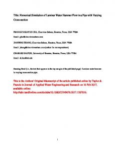
Fig. 1 Schematic figure of initial bubble location Table 1 simulation conditions of periodic flow Case 1 2 3 4
fG0 (%) 0 0.1 0.1 0.1
Initial bubble location + 0