VIII International Conference on Computational Plasticity COMPLAS VIII E. Oñate and D. R. J. Owen (Eds) CIMNE, Barcelona, 2005
ON PARTICLE FINITE ELEMENT METHODS IN SOLID MECHANICS PROBLEMS J. Oliver*, J.C. Cante† and C. Gonzalez*
†
*Technical University of Catalonia (UPC)
International Center for Numerical Methods in Engineering (CIMNE) Campus Nord UPC, Edifici-C-1, c/Jordi Girona 1-3 08034 Barcelona, Spain e-mail:
[email protected], web page: http://www.cimne.upc.es/personales/oliver/
Key words: particle finite element methods, contact interfaces, forming processes. Summary. The paper focuses the application of the Particle Finite Element Methods (PFEM) to modeling forming processes in solid mechanics. The fundamentals of the PFEM are briefly introduced, and, then, a contact modeling strategy, based on the anticipation of the contacting boundaries and the construction of a contact interface, is described. Application to filling and machining processes is finally presented. 1
INTRODUCTION
In the last years particle finite element methods (PFEM) have gained considerable interest in the CFD community as a procedure to tackle fluid mechanics problems in a solid mechanics format: i.e. using Lagrangean descriptions of the motion of the continuum medium 2-7 . Their main advantages are found in modeling confined fluids exhibiting moving free surfaces. There, the limited character of the particle displacement makes possible a Lagrangean description which, in turn, facilitates the tracking and modeling of the appearing free surfaces. Here we consider the possibilities of the application of that method in those solid mechanics problems that share with fluids some of the above features i.e.: large deformations and rapidly changing free boundaries. A typical example of that kind of problems is forming processes. 2
FUNDAMENTALS OF THE PARTICLE FINITE ELEMENT METHOD.
The particle finite element methods emerged as a natural result of previous explorations in the context of the meshless methods 6. They can be characterized by the following ingredients: 1) The use of a Lagrangean format for describing the motion. A selected cloud of particles of infinitesimal size (material points) are tracked along the motion to describe the continuum medium properties evolution (position, displacement, velocities, strain, stresses, internal variables etc.). When necessary, the properties of the remaining particles of the continuum
.J. Oliver, J.C. Cante and C. Gonzalez
medium are obtained by interpolation of the properties at points of that cloud. 2) Numerical computations are done on the basis of a finite element mesh that is constructed at every time step on the basis of the particle positions. Then, Delaunay triangulations, allowing the construction of a finite element mesh for a given sets of nodes, emerge as a suitable meshing procedure 1. 3) The use of a boundary recognition procedure to identify what particles of the cloud define an external (or internal) boundary. The so-called alpha-shape method 1 constitutes a suitable strategy for this purpose. It essentially consists of eliminating those elements of the triangulation that can be inserted into an empty circle (not including other particles of the cloud) of size larger then a given parameter (the alpha-shape parameter). The nodes (particles) of those eliminated triangles can be then identified as the boundary particles. Large values of the alpha-shape parameter result in a boundary which is the convex hull of the cloud. Small values of the alpha-shape parameter return a boundary constituted of all the particles of the cloud. For a uniformly distributed cloud of particles (with typical separation h ) alpha-shape values of 1.1h − 1.5h provide a good estimation of the actual boundary. Ω n +1 Ω t =t n = {X i ; i : 1K n part }
Xi
u n +1 Non linear incremental problem
Initial data
{v n , a n , qn }
M n +1 ⋅ a n +1 + Fnint+1 (u n +1 ) − Fnext+1 (u n +1 ) = 0 u n +1 = u n + ∆tv n + 12 ∆t 2 [(1 − 2β) an + 2βan +1 ] v n +1 = v n + ∆t [(1 − γ )a n + γa n +1 ]
[
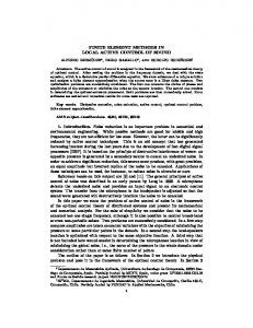
Figure 1. Incremental non-linear problem at time step t n , t n +1
u n +1
]
The numerical procedure at a given time t n +1 consists of the following stages (see Figure 1): a) constructing a Delaunay triangulation on the basis of the particle positions at time t n (configuration Ω n ), b) identification of the boundary of Ω n , and subsequent elimination of the external triangles, via alpha-shape methods, resulting in a triangle finite element mesh, c) solving the corresponding discrete incremental non-linear finite element problem, in a standard Lagrangean way referred to configuration Ω n , and obtaining all the required nodal (particle) variables of the problem: displacements u n+1 , velocities v n +1 , accelerations a n+1 , stresses σ n+1 , internal variables q n+1 etc. , d) updating the positions of the particles according to the displacements of the previous time step resulting in the configuration Ω n +1 .
2
.J. Oliver, J.C. Cante and C. Gonzalez
3
A CONTACT STRATEGY BASED ON AN ANTICIPATED CONTACT INTERFACE.
One of the main difficulties found in standard contact algorithms is the identification of the interacting parts of two contacting bodies (master-slave based algorithms). The previous PFEM setting provides a very interesting feature to be exploited in this sense: the possibility of anticipating the contact boundaries and of imposing the corresponding contact constraints in a diffuse manner, without the necessity of a precise identification of the contact topologies. The method is sketched in Figure 2. Class 1: forming material Class 2: tool Class 3: interface σ
Contact / friction model
p
lc σ
ε = [( x ( p ) − x ( q )) ⋅ n − g ] lc
Κ
τ
n t
q
g
ε
K σ = K (ε) ε ; K (ε) = 0 τ = µ σ sign ( v P ⋅ t )
ε