Optimal Exponential Synchronization of Chaotic Systems with Multiple

Hindawi Publishing Corporation Abstract and Applied Analysis Volume 2013, Article ID 742821, 19 pages http://dx.doi.org/10.1155/2013/742821

Research Article Optimal Exponential Synchronization of Chaotic Systems with Multiple Time Delays via Fuzzy Control Feng-Hsiag Hsiao Department of Electrical Engineering, National University of Tainan, No. 33, Section 2, Shu Lin Street, Tainan 700, Taiwan Correspondence should be addressed to Feng-Hsiag Hsiao; [email protected] Received 15 January 2013; Revised 26 April 2013; Accepted 28 April 2013 Academic Editor: Ryan Loxton Copyright © 2013 Feng-Hsiag Hsiao. This is an open access article distributed under the Creative Commons Attribution License, which permits unrestricted use, distribution, and reproduction in any medium, provided the original work is properly cited. This study presents an effective approach to realize the optimal H ∞ exponential synchronization of multiple time-delay chaotic (MTDC) systems. First, a neural network (NN) model is employed to approximate the MTDC system. Then, a linear differential inclusion (LDI) state-space representation is established for the dynamics of the NN model. Based on this LDI state-space representation, this study proposes a delay-dependent exponential stability criterion of the error system derived in terms of Lyapunov’s direct method to ensure that the trajectories of the slave system can approach those of the master system. Subsequently, the stability condition of this criterion is reformulated into a linear matrix inequality (LMI). Based on the LMI, a fuzzy controller is synthesized not only to realize the exponential synchronization but also to achieve the optimal H ∞ performance by minimizing the disturbance attenuation level. Finally, a numerical example with simulations is provided to illustrate the concepts discussed throughout this work.

1. Introduction In practice, due to information transmission, time delays naturally exist in many systems. The existence of time delay is frequently a source of instability and is encountered in various engineering systems [1–5]. Consequently, the problem of stability analysis in time-delay systems remains a major focus of researchers wishing to inspect the properties of such systems. Since chaotic phenomenon in time-delay systems was first found by Mackey and Glass [6], there has been increasing interest in time-delay chaotic systems. Chaos is a wellknown nonlinear phenomenon, and it is irregular, seemingly random and extremely sensitive to initial conditions [7]. Based on these properties, chaos has received a great deal of interest among scientists from various research fields [8– 12]. One of its research fields for communication, chaotic synchronization, has been investigated extensively.

The chaotic synchronization proposed by Pecora and Carroll in 1990 [13] is intended to control one chaotic system to follow another. Since the introduction of this concept, various synchronization approaches, such as nonlinear feedback control [14] and adaptive control [15], have been widely developed in the past two decades. Chaos synchronization can be applied in the vast areas of physics and engineering science, especially in secure communication [16]. Therefore, chaotic synchronization has become a popular study [14–23]. In real physical systems, some noises or disturbances always exist that may cause instability and thereby destroy the synchronization performance. Hence, how to reduce the effect of external disturbances in synchronization process for chaotic systems is an important issue [24, 25]. The 𝐻∞ control has been conferred for synchronization in chaotic systems over the last few years [24–28]. And the 𝐻∞ synchronization problem was also investigated extensively for timedelay chaotic systems (see, e.g., [25, 29–31]). Accordingly,

2

Abstract and Applied Analysis

the objective of this study is to realize the exponential synchronization of multiple time-delay chaotic (MTDC) systems, and at the same time the effect of external disturbance on control performance is attenuated to a minimum level. Neural-network- (NN-) based modeling has become an active research field in the past few years due to its unique merits in solving complex nonlinear system identification and control problems [32–37]. Over the past decade, fuzzy control has rapidly developed in both the academic and industrial communities and there have been many successful applications. Despite the successes of fuzzy control, it has become evident that many basic problems remain to be solved. Stability analysis and systematic design are certainly among the most important issues for fuzzy control systems. Lately, there have been significant research efforts devoted to these issues (see [38–41]). However, all of them neglect the modeling errors between nonlinear systems and fuzzy models. The existence of modeling errors may be a potential source of instability for control designs based on the assumption that the fuzzy model exactly matches the nonlinear plant [42]. Recently, Kiriakidis [42], Chen et al. [43, 44], and Cao et al. [45, 46] proposed novel approaches to overcome the influence of modeling errors in the field of model-based fuzzy control for nonlinear systems. Consequently, an effective method is proposed via neural-network- (NN-) based technique to realize the optimal 𝐻∞ exponential synchronization of multiple time-delay chaotic (MTDC) systems in this study. Based on the above, the trajectories of slave systems can approach those of master systems and the effect of external disturbance on control performance is attenuated to a minimum level. This study is organized as follows. The system description is arranged in Section 2. In Section 3, a robustness design of fuzzy controllers is proposed to realize the optimal 𝐻∞ exponential synchronization. The design algorithm is shown in Section 4. In Section 5, the effectiveness of the proposed approach is illustrated by a numerical example. Finally, the conclusions are drawn in Section 6.

2. System Description Consider a pair of multiple time-delay chaotic (MTDC) systems in master-slave configuration. The dynamics of the master system (𝑁𝑚 ) and slave system (𝑁𝑠 ) are described as follows:

𝑥1 (𝑡) .. . 𝑥𝛿 (𝑡) 𝑥1 (𝑡 − 𝜏1 ) .. . 𝑥1 (𝑡 − 𝜏𝑚 )

𝑥2 (𝑡 − 𝜏1 ) .. .

.. .

𝑇(·)

.

x1 (t)

···

.. .

.. .

.. . .

x𝛿 (t)

···

𝑥𝛿 (𝑡 − 𝜏𝑚 )

Figure 1: An NN model.

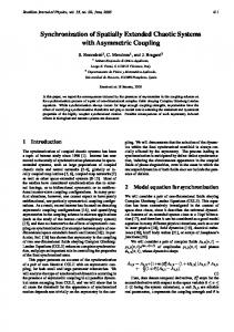
In this section, a neural network (NN) model is first established to approximate the MTDC system. The dynamics of the NN model are then converted into a linear differential inclusion (LDI) state-space representation. Finally, on the basis of the LDI state-space representation, a fuzzy controller is synthesized to realize the synchronization of MTDC systems. 2.1. Neural Network (NN) Model. The MTDC system can be approximated by an NN model, as shown in Figure 1, that has 𝑆 layers with 𝐽𝜎 (𝜎 = 1, 2, . . . , 𝑆) neurons for each layer, in which 𝑥1 (𝑡) ∼ 𝑥𝛿 (𝑡) are the state variables and 𝑥1 (𝑡 − 𝜏1 ) ∼ 𝑥1 (𝑡 − 𝜏𝑚 ), 𝑥2 (𝑡 − 𝜏1 ) ∼ 𝑥𝛿 (𝑡 − 𝜏𝑚 ) are the state variables with delays. To distinguish among these layers, the superscripts are used for identifying the layers. Specifically, we append the number of the layer as a superscript to the names for each of these variables. Thus, the weight matrix for the 𝜎th layer is written as 𝑊𝜎 . Moreover, it is assumed that V𝜍𝜎 (𝑡) (𝜍 = 1, 2, . . . , 𝐽𝜎 ; 𝜎 = 1, 2, . . . , 𝑆) is the net input and 𝑇(V𝜍𝜎 (𝑡)) is the transfer function of the neuron. Subsequently, the transfer function vector of the 𝜎th layer is defined as

𝑇

Ψ𝜎 (V𝜍𝜎 (𝑡)) ≡ [𝑇 (V1𝜎 (𝑡)) 𝑇 (V2𝜎 (𝑡)) ⋅ ⋅ ⋅ 𝑇 (V𝐽𝜎𝜎 (𝑡))] ,

(3)

𝜎 = 1, 2, . . . , 𝑆,

𝑚

𝑁𝑚 : 𝑋̇ (𝑡) = 𝑓 (𝑋 (𝑡)) + ∑ 𝐻𝑘 (𝑋 (𝑡 − 𝜏𝑘 )) ,

∑

(1)

𝑘 =1

𝑚

̂̇ (𝑡) = 𝑓 (𝑋 ̂ (𝑡)) + ∑ 𝐻𝑘 (𝑋 ̂ (𝑡 − 𝜏𝑘 )) + 𝐵𝑈 (𝑡) + 𝜕 (𝑡) , 𝑁𝑠 : 𝑋 𝑘 =1

(2) where 𝑓(⋅) and 𝐻𝑘 (⋅) are the nonlinear vector-valued functions, 𝜕(𝑡) denotes the external disturbance, 𝜏𝑘 (𝑘 = 1, 2, . . . , 𝑚) are the time delays, and 𝑈(𝑡) is the control input. ̂ are the state vectors of 𝑁𝑚 and 𝑁𝑠 , Moreover, 𝑋(𝑡) and 𝑋(𝑡) respectively.

where 𝑇(V𝜍𝜎 (𝑡)) (𝜍 = 1, 2, . . . , 𝐽𝜎 ) is the transfer function of the 𝜍th neuron. The final output of NN model can then be inferred as follows: 𝑋̇ (𝑡) = Ψ𝑆 (𝑊𝑆 Ψ𝑆−1 (𝑊𝑆−1 Ψ𝑆−2 × (⋅ ⋅ ⋅ Ψ2 (𝑊2 Ψ1 (𝑊1 Λ (𝑡))) ⋅ ⋅ ⋅ ))) , (4)


3

where Λ𝑇 (𝑡) = [𝑋𝑇 (𝑡) 𝑋𝑇 (𝑡 − 𝜏𝑘 )]

(5)

with

𝜎 𝜎 𝜎 𝜎 + ℎ𝜍1 ) V𝜍𝜎 (𝑡) 𝑇 (V𝜍𝜎 (𝑡)) = (ℎ𝜍0 (𝑡) 𝑔𝜍0 (𝑡) 𝑔𝜍1

𝑇

𝑋 (𝑡) = [𝑥1 (𝑡) 𝑥2 (𝑡) ⋅ ⋅ ⋅ 𝑥𝛿 (𝑡)] , 𝑋 (𝑡 − 𝜏𝑘 ) = [𝑥1 (𝑡 − 𝜏1 ) ⋅ ⋅ ⋅ 𝑥1 (𝑡 − 𝜏𝑚 ) 𝑥2 (𝑡 − 𝜏1 ) ⋅ ⋅ ⋅ 𝑥𝛿 (𝑡 − 𝜏𝑚 )]

𝑇

Moreover, based on the interpolation method, the transfer function 𝑇(V𝜍𝜎 (𝑡)) can be represented as follows [47]:

=

(6)

for 𝑘 = 1, 2, . . . , 𝑚.

2.2. Linear Differential Inclusion (LDI). To deal with the synchronization problem of MTDC systems, this study establishes the following LDI state-space representation for the dynamics of the NN model, described as [47, 48]:

𝜙

(11) (𝑡) ,

𝜎 (𝑡) ∈ [0, 1] and where the interpolation coefficients ℎ𝜍𝜑

𝜎 (𝑡) = 1. Equations (3) and (11) show that ∑1𝜑 = 0 ℎ𝜍𝜑

(7)

1

1

𝜑1 = 0

𝜑2 = 0

𝜎 𝜎 𝜎 𝜎 = [( ∑ ℎ1𝜑 ) V1𝜎 (𝑡) ( ∑ ℎ2𝜑 ) (𝑡) 𝑔1𝜑 (𝑡) 𝑔2𝜑 1 1 2 2

𝑖 =1

where 𝜙 is a positive integer, 𝑎(𝑡) is a vector signifying the ̃𝑖 (𝑖 = 1, 2, . . . , 𝜙) are dependence of ℎ𝑖 (⋅) on its elements, 𝐴 constant matrices, and 𝑂(𝑡) = [𝑜1 (𝑡) 𝑜2 (𝑡) ⋅ ⋅ ⋅ 𝑜ℵ (𝑡)]𝑇 . Furthermore, it is assumed that ℎ𝑖 (𝑎(𝑡)) ≥ 0 and 𝜙 ∑𝑖 =1 ℎ𝑖 (𝑎(𝑡)) = 1. Based on the properties of LDI, without loss of generality, we can use ℎ𝑖 (𝑡) instead of ℎ𝑖 (𝑎(𝑡)). The following procedure represents the dynamics of the NN model (4) by LDI state-space representation [47]. To begin with, notice that the output 𝑇(V𝜍𝜎 (𝑡)) satisfies 𝜎 𝜎 𝜎 𝜎 𝑔𝜍0 V𝜍 (𝑡) ≤ 𝑇 (V𝜍𝜎 (𝑡)) ≤ 𝑔𝜍1 V𝜍 (𝑡) ,

V𝜍𝜎 (𝑡) ≥ 0,

𝜎 𝜎 𝜎 𝜎 𝑔𝜍1 V𝜍 (𝑡) ≤ 𝑇 (V𝜍𝜎 (𝑡)) ≤ 𝑔𝜍0 V𝜍 (𝑡) ,

V𝜍𝜎 (𝑡) < 0,

(8)

𝜎 𝜎 where 𝑔𝜍0 and 𝑔𝜍1 denote the minimum and the maximum of the derivative of 𝑇(V𝜍𝜎 (𝑡)), respectively, and are given in the following:

× V2𝜎

1

1

𝑝=0

1

2 × (𝑊𝑆 [⋅ ⋅ ⋅ [ ∑ ℎ𝜍𝑛 (𝑡) 𝐺2 𝑛=0

1

1 × (𝑊2 [ ∑ ℎ𝜍𝑏 (𝑡) 𝐺1 𝑏=0

× (𝑊1 Λ (𝑡)) ])] ⋅ ⋅ ⋅ ])

Subsequently, the min-max matrix 𝐺𝜎 of the 𝜎th layer is defined as follows:

0

] ] ] ] ]. ] ] 0 ]

d 0 𝑔𝐽𝜎𝜎 𝜑𝐽 ]

(𝑡)] . ] (12)

𝑆 𝑋̇ (𝑡) = ∑ ℎ𝜍𝑝 (𝑡) 𝐺𝑆

when 𝜑 = 1.

0 0 .. .

(𝑡) 𝑔𝐽𝜎𝜎 𝜑𝐽 ) V𝐽𝜎𝜎

Therefore, the final output of the NN model (4) can be reformulated as follows:

(9)

⋅⋅⋅ d

𝑇

(𝑡) ⋅ ⋅ ⋅ ( ∑ ℎ𝐽𝜎𝜎 𝜑𝐽 𝜑𝐽 = 0

when 𝜑 = 0,

𝜎 0 0 𝑔1𝜑 1 [ 0 𝑔𝜎 0 2𝜑2 [ [ [ 𝜎 𝜎 0 𝑔3𝜑3 𝐺𝜎 ≡ diag [𝑔𝜍𝜑 ]=[ 0 𝜍 [ . [ . [ . d 0 0 0 ⋅ ⋅⋅ [

𝜎 ) V𝜍𝜎 (𝑡) 𝑔𝜍𝜑

𝑇

̃𝑖 , 𝐴 (𝑎 (𝑡)) = ∑ ℎ𝑖 (𝑎 (𝑡)) 𝐴

𝜎 𝑔𝜍𝜑 =

𝜎 ( ∑ ℎ𝜍𝜑 𝜑 =0

Ψ𝜎 (V𝜍𝜎 (𝑡)) ≡ [𝑇 (V1𝜎 (𝑡)) 𝑇 (V2𝜎 (𝑡)) ⋅ ⋅ ⋅ 𝑇 (V𝐽𝜎𝜎 (𝑡))]

𝑂̇ (𝑡) = 𝐴 (𝑎 (𝑡)) 𝑂 (𝑡) ,

𝑑𝑇 (V𝜍𝜎 (𝑡)) { { min { { { V 𝑑V𝜍𝜎 (𝑡) { { 𝑑𝑇 (V𝜍𝜎 (𝑡)) { { {max 𝑑V𝜍𝜎 (𝑡) { V

1

1

1

1

𝑆 2 1 = ∑ ⋅ ⋅ ⋅ ∑ ∑ ℎ𝜍𝑝 (𝑡) ⋅ ⋅ ⋅ ℎ𝜍𝑛 (𝑡) ℎ𝜍𝑏 (𝑡) 𝐺𝑆 𝑊𝑆 𝑝=0

𝑛=0 𝑏=0

⋅ ⋅ ⋅ 𝐺2 𝑊2 𝐺1 𝑊1 Λ (𝑡) (10)

𝜎 𝜎 Λ (𝑡) , = ∑ℎ𝜍Ω (𝑡) 𝐶Ω Ω

(13)

4


where 1

1

1

1

𝑏=0

𝑏1 = 0

𝑏2 = 0

𝑏𝐽 = 0

1

1

1

1

𝑛=0

𝑛1 = 0

𝑛2 = 0

𝑛𝐽 = 0

The fuzzy controller takes the following form: Control Rule 𝑙:

1 1 1 ∑ ℎ𝜍𝑏 (𝑡) ≡ ∑ ℎ1𝑏 (𝑡) ∑ ℎ2𝑏 (𝑡) ⋅ ⋅ ⋅ ∑ ℎ𝐽11 𝑏𝐽 (𝑡) , 1 2

IF 𝑒1 (𝑡) is 𝑀𝑙1 and ⋅ ⋅ ⋅ and 𝑒𝛿 (𝑡) is 𝑀𝑙𝛿 THEN 𝑈 (𝑡) = −𝐾𝑙 𝐸 (𝑡) ,

2 2 2 ∑ ℎ𝜍𝑛 (𝑡) ≡ ∑ ℎ1𝑛 (𝑡) ∑ ℎ2𝑛 (𝑡) ⋅ ⋅ ⋅ ∑ ℎ𝐽22 𝑛𝐽 (𝑡) , 1 2

.. .

(14)

1

1

1

1

𝑝=0

𝑝1 = 0

𝑝2 = 0

𝑝𝐽 = 0

where 𝑙 = 1, 2, . . . , 𝜌, and 𝜌 is the number of IF-THEN rules of the fuzzy controller and 𝑀𝑙𝜂 (𝜂 = 1, 2, . . . , 𝛿) are the fuzzy sets. Hence, the final output of this fuzzy controller can be inferred as follows:

𝑆 𝑆 𝑆 ∑ ℎ𝜍𝑝 (𝑡) ≡ ∑ ℎ1𝑝 (𝑡) ∑ ℎ2𝑝 (𝑡) ⋅ ⋅ ⋅ ∑ ℎ𝐽𝑆𝑆 𝑝𝐽 (𝑡) , 1 2 1

1

𝜌

𝑝=0

𝜌

∑𝑙 =1 𝑤𝑙 (𝑡)

1

= − ∑ ℎ𝑙 (𝑡) 𝐾𝑙 𝐸 (𝑡) , 𝑙 =1

𝜎 𝐶Ω ≡ 𝐺𝑆 𝑊𝑆 ⋅ ⋅ ⋅ 𝐺2 𝑊2 𝐺1 𝑊1

and 𝑏𝜍 , 𝑛𝜍 , 𝑝𝜍 (𝜍 = 1, 2, . . . , 𝐽𝜎 ) represent the variables 𝜑 of the 𝜍th neuron of the first, second, and the Sth layer, respectively. Finally, according to (7), the dynamics of the NN model (13) can be rewritten as the following LDI state-space representation: 𝜙

𝑋̇ (𝑡) = ∑ ℎ𝑖 (𝑡) 𝐶𝑖 Λ (𝑡) ,

(15)

𝑖 =1

𝜙

where ℎ𝑖 (𝑡) ≥ 0, ∑𝑖 =1 ℎ𝑖 (𝑡) = 1, 𝜙 is a positive integer, and 𝐶𝑖 is a constant matrix with appropriate dimension associated 𝜎 . Moreover, the LDI state-space representation (15) with 𝐶Ω can be rearranged as follows: 𝜙

𝑚

𝑖 =1

𝑘 =1

𝑋̇ (𝑡) = ∑ ℎ𝑖 (𝑡) {𝐴 𝑖 𝑋 (𝑡) + ∑ 𝐴𝑖𝑘 𝑋 (𝑡 − 𝜏𝑘 )} ,

(16)

where 𝐴 𝑖 and 𝐴𝑖𝑘 are the partitions of 𝐶𝑖 corresponding to the partitions of Λ𝑇 (𝑡). From the above, the NN models of the master and slave chaotic systems are described by the following LDI statespace representations (17) and (18), respectively: 𝜙

𝑚

𝑖 =1

𝑘 =1

(20)

𝜌

𝑛=0 𝑏=0

𝜍 = 1, 2, . . . , 𝐽𝜎 ;

− ∑𝑙 =1 𝑤𝑙 (𝑡) 𝐾𝑙 𝐸 (𝑡)

𝑈 (𝑡) =

𝜎 𝑆 2 1 ∑ℎ𝜍Ω (𝑡) ≡ ∑ ⋅ ⋅ ⋅ ∑ ∑ ℎ𝜍𝑝 (𝑡) ⋅ ⋅ ⋅ ℎ𝜍𝑛 (𝑡) ℎ𝜍𝑏 (𝑡) , Ω

𝜌

with 𝑤𝑙 (𝑡) ≡ ∏𝛿𝜂 =1 𝑀𝑙𝜂 (𝑒𝜂 (𝑡)), ℎ𝑙 (𝑡) ≡ 𝑤𝑙 (𝑡)/(∑𝑙 =1 𝑤𝑙 (𝑡)), in which 𝑀𝑙𝜂 (𝑒𝜂 (𝑡)) is the grade of membership of 𝑒𝜂 (𝑡) in 𝑀𝑙𝜂 . In this study, it is also assumed that 𝑤𝑙 (𝑡) ≥ 0 (𝑙 = 𝜌 1, 2, . . . , 𝜌) and ∑𝑙 =1 𝑤𝑙 (𝑡) > 0 for all 𝑡. Therefore, ℎ𝑙 (𝑡) ≥ 0 𝜌 and ∑𝑙 =1 ℎ𝑙 (𝑡) = 1 for all 𝑡.

3. Robustness Design of Chaotic Synchronization and Stability Analysis In this section, the synchronization of multiple time-delay chaotic (MTDC) systems is examined under the influence of modeling error. 3.1. Error Systems. From (1) and (2), the synchronizâ tion error is defined as 𝐸(𝑡) ≡ 𝑋(𝑡) − 𝑋(𝑡) = [𝑒1 (𝑡), 𝑒2 (𝑡), . . . , 𝑒𝛿 (𝑡)]𝑇 and then the dynamics of the error system under the fuzzy control (20) can be described as follows: 𝐸̇ (𝑡) = Γ̂ + 𝜕 (𝑡) − Γ 𝜙

𝜙

𝜌

+ ∑ ∑ ∑ ℎ𝑖 (𝑡) ̂ℎ𝑗 (𝑡) ℎ𝑙 (𝑡) 𝑖 =1 𝑗 =1 𝑙 =1

Master: 𝑋̇ (𝑡) = ∑ ℎ𝑖 (𝑡) {𝐴 𝑖 𝑋 (𝑡) + ∑ 𝐴𝑖𝑘 𝑋 (𝑡 − 𝜏𝑘 )}

̂𝑗 − 𝐴 𝑖 ) 𝑋 ̂ (𝑡) × {𝐷𝑖𝑙 𝐸 (𝑡) + (𝐴

(17) 𝜙

𝑚

𝑗 =1

𝑘 =1

̂ 𝑋 ̂̇ (𝑡) = ∑ ̂ℎ𝑗 (𝑡) [𝐴 ̂ (𝑡) + ∑ 𝐴 ̂ ̂𝑗 𝑋 Slave: 𝑋 𝑗𝑘 (𝑡 − 𝜏𝑘 )]

(19)

𝑚

̂ − 𝐴 )𝑋 ̂ (𝑡 − 𝜏𝑘 ) + ∑ (𝐴 𝑗𝑘 𝑖𝑘 𝑘 =1

(18)

𝑚

+ 𝐵𝑈 (𝑡) .

+ ∑ 𝐴𝑖𝑘 𝐸 (𝑡 − 𝜏𝑘 )} 𝑘 =1

2.3. Fuzzy Controller. According to the control scheme, a fuzzy controller is utilized to make the slave system synchronize with the master system.

𝜙

𝜙

𝜌

− ∑ ∑ ∑ ℎ𝑖 (𝑡) ̂ℎ𝑗 (𝑡) ℎ𝑙 (𝑡) 𝑖 =1 𝑗 =1 𝑙 =1


5 where 𝑌 is the specified structured bounding matrix and ‖𝜅𝑖𝑙 ‖ ≤ 1 for 𝑖 = 1, 2, . . . , 𝜙; 𝑙 = 1, 2, . . . , 𝜌. Equations (24) and (25) show that

̂𝑗 − 𝐴 𝑖 ) 𝑋 ̂ (𝑡) × {𝐷𝑖𝑙 𝐸 (𝑡) + (𝐴 𝑚

̂ − 𝐴 )𝑋 ̂ (𝑡 − 𝜏𝑘 ) + ∑ (𝐴 𝑗𝑘 𝑖𝑘

Φ (𝑡) Φ (𝑡) ≤ [ ∑ ∑ ℎ𝑖 (𝑡) ℎ𝑙 (𝑡) Δ𝑌𝑖𝑙 𝐸 (𝑡)]

𝑘 =1

𝑖 =1 𝑙 =1

𝑚

+ ∑ 𝐴𝑖𝑘 𝐸 (𝑡 − 𝜏𝑘 )}

𝜌

𝜙

× [ ∑ ∑ ℎ𝑖 (𝑡) ℎ𝑙 (𝑡) Δ𝑌𝑖𝑙 𝐸 (𝑡)]

𝑘 =1

𝜙

𝑇

𝜌

𝜙

𝑇

𝑖 =1 𝑙 =1

𝜌

= ∑ ∑ ℎ𝑖 (𝑡) ℎ𝑙 (𝑡)

𝜙

𝜌

󵄩 󵄩 ≤ ∑ ∑ ℎ𝑖 (𝑡) ℎ𝑙 (𝑡) ‖𝑌𝐸 (𝑡)‖ 󵄩󵄩󵄩𝜅𝑖𝑙 󵄩󵄩󵄩

𝑖 =1 𝑙 =1

(26)

𝑖 =1 𝑙 =1

𝑚

× {𝐷𝑖𝑙 𝐸 (𝑡) + ∑ 𝐴𝑖𝑘 𝐸 (𝑡 − 𝜏𝑘 )}

𝜙

𝜌

󵄩 󵄩 × ∑ ∑ ℎ𝑖 (𝑡) ℎ𝑙 (𝑡) 󵄩󵄩󵄩𝜅𝑖𝑙 󵄩󵄩󵄩 ‖𝑌𝐸 (𝑡)‖

𝑘 =1

𝑖 =1 𝑙 =1

+ 𝜕 (𝑡) + Φ (𝑡) , (21)

≤ [𝑌𝐸 (𝑡)]𝑇 [𝑌𝐸 (𝑡)] ≤ 𝐸𝑇 (𝑡) 𝑌𝑇 𝑌𝐸 (𝑡) . Namely, Φ(𝑡) is bounded by the specified structured bounding matrix 𝑌.

where 𝐷𝑖𝑙 ≡ 𝐴 𝑖 − 𝐵𝐾𝑙 ,

Remark 1 (see [43]). The following simple example describes the procedures for determining 𝜅𝑖𝑙 and 𝑌. First, assume that the possible bounds for all elements in Δ𝑌𝑖𝑙 are

𝑚

̂ (𝑡)) + ∑ 𝐻𝑘 (𝑋 ̂ (𝑡 − 𝜏𝑘 )) + 𝑈 (𝑡) , Γ̂ ≡ 𝑓 (𝑋 𝑘 =1

𝑚

(22)

Γ ≡ 𝑓 (𝑋 (𝑡)) + ∑ 𝐻𝑘 (𝑋 (𝑡 − 𝜏𝑘 )) 𝑘 =1

with

Δ𝑦𝑖𝑙11 Δ𝑦𝑖𝑙12 Δ𝑦𝑖𝑙13 ] [ 21 [Δ𝑦 Δ𝑦22 Δ𝑦23 ] ], [ 𝑖𝑙 𝑖𝑙 𝑖𝑙 Δ𝑌𝑖𝑙 = [ ] ] [ 31 32 33 Δ𝑦𝑖𝑙 Δ𝑦𝑖𝑙 Δ𝑦𝑖𝑙 ] [ 𝑞𝑠

𝜌 𝑙 =1

𝜌

Φ (𝑡) ≡ Γ̂ − Γ − { ∑ ∑ ℎ𝑖 (𝑡) ℎ𝑙 (𝑡) [𝐷𝑖𝑙 𝐸 (𝑡)

(23)

𝑖 =1 𝑙 =1 𝑚

𝑘 =1

Suppose that there exists a bounding matrix Δ𝑌𝑖𝑙 such that

(24)

for the trajectory 𝐸(𝑡), and the bounding matrix Δ𝑌𝑖𝑙 can be described as follows: Δ𝑌𝑖𝑙 = 𝜅𝑖𝑙 𝑌,

𝜅𝑖𝑙11 0 0 𝑦11 𝑦12 𝑦13 22 Δ𝑌𝑖𝑙 = [ 0 𝜅𝑖𝑙 0 ] [𝑦21 𝑦22 𝑦23 ] = 𝜅𝑖𝑙 𝑌, 33 31 32 33 [ 0 0 𝜅𝑖𝑙 ] [𝑦 𝑦 𝑦 ]

(28)

𝑞𝑞

where −1 ≤ 𝜅𝑖𝑙 ≤ 1 for 𝑞 = 1, 2, 3. Notice that 𝜅𝑖𝑙 can be chosen by other forms as long as ‖𝜅𝑖𝑙 ‖ ≤ 1. Then, we check the validity of (24) in the simulation. If it is not satisfied, we can expand the bounds for all elements in Δ𝑌𝑖𝑙 and repeat the design procedure until (24) holds.

+ ∑ 𝐴𝑖𝑘 𝐸 (𝑡 − 𝜏𝑘 )]} .

󵄩󵄩 𝜙 𝜌 󵄩󵄩 󵄩󵄩 󵄩󵄩 󵄩 ‖Φ (𝑡)‖ ≤ 󵄩󵄩󵄩 ∑ ∑ ℎ𝑖 (𝑡) ℎ𝑙 (𝑡) Δ𝑌𝑖𝑙 𝐸 (𝑡)󵄩󵄩󵄩󵄩 󵄩󵄩𝑖 =1 𝑙 =1 󵄩󵄩 󵄩 󵄩

𝑞𝑠

where −𝑦𝑞𝑠 ≤ Δ𝑦𝑖𝑙 ≤ 𝑦𝑞𝑠 for some 𝑦𝑖𝑙 with q, 𝑠 = 1, 2, 3; 𝑖 = 1, 2, . . . , 𝜙; and 𝑙 = 1, 2, . . . , 𝜌. A possible description for the bounding matrix Δ𝑌𝑖𝑙 is

𝑈 (𝑡) = − ∑ ℎ𝑙 (𝑡) 𝐾𝑙 𝐸 (𝑡) , 𝜙

(27)

(25)

3.2. Delay-Dependent Stability Criterion for Exponential 𝐻∞ Synchronization. In this subsection, a delay-dependent criterion is proposed to guarantee the exponential stability of the error system described in (21). Moreover, in real physical systems, some noises or disturbances always exist that may cause instability and thereby destroy the synchronization performance. To reduce the effect of the external disturbance, an optimal 𝐻∞ scheme is used to design the fuzzy control so that the effect of external disturbance on control performance can be attenuated to a minimum level. In other words, in this study, the fuzzy controller (20) not only realizes exponential synchronization but also achieves the optimal 𝐻∞ control performance.

6


Prior to the examination of the stability of the error system, some definitions and a lemma are given next.

where 𝐷𝑖𝑙 ≡ 𝐴 𝑖 − 𝐵𝐾𝑙 for 𝑖 = 1, 2, . . . , 𝜙; 𝑘 = 1, 2, . . . , 𝑚 and 𝑙 = 1, 2, . . . , 𝜌.

Definition 2 (see [49]). The slave system (2) can exponentially synchronize with the master system (1) (i.e., the error system (21) is exponentially stable) if there exist two positive numbers 𝛼 and 𝛽 such that the synchronization error satisfies

Proof. See the appendix.

‖𝐸 (𝑡)‖ ≤ 𝛼 exp (−𝛽 (𝑡 − 𝑡0 )) ,

∀𝑡 ≥ 0.

(29)

The positive number 𝛽 is called the exponential convergence rate. Definition 3 (see [24–28]). The master system (1) and slave system (2) are said to be exponential 𝐻∞ synchronization if the following conditions are satisfied: (i) in the case of 𝜕(𝑡) = 0, the error system (21) is exponentially stable, (ii) under the zero initial conditions (i.e., 𝐸(𝑡) = 0 for 𝑡 ∈ [−𝜏max , 0], in which 𝜏max is the maximal value of 𝜏𝑘 ’s) and a given constant 𝛾 > 0, the following condition holds: ∞

∞

0

0

Remark 6. Based on (24), Φ(𝑡) is assumed to be bounded by the specified structured bounding matrix 𝑌 and then the larger Φ(𝑡) results in larger 𝑌. Since the matrices Δ 𝑖𝑙 must be negative definite to meet the stability condition (32b), the larger 𝑌 will make Theorem 5 more difficult to satisfy. Corollary 7. Equations (32b) and (32c) can be reformulated into LMIs via the following procedure. By introducing the new variables 𝑄 = 𝑃−1 , 𝐹𝑙 = 𝐾𝑙 𝑄, and 𝜓𝑘 = 𝑄𝜓𝑘 𝑄, (32b) and (32c) can be rewritten as follows: 𝑚

∑ 𝜏𝑘 {𝑄𝐴𝑇𝑖 − 𝐹𝑙𝑇 𝐵𝑇 + 𝐴 𝑖 𝑄 − 𝐵𝐹𝑙 }

𝑘 =1

𝑚

+ ∑ 𝜏𝑘2 (𝑐−1 + 𝑛−1 + 𝑚𝑎−1 ) 𝐼 𝑘 =1

Θ (𝐸 (𝑡) , 𝜕 (𝑡)) = ∫ 𝐸𝑇 (𝑡) 𝐸 (𝑡) 𝑑𝑡 − 𝛾2 ∫ 𝜕𝑇 (𝑡) 𝜕 (𝑡) 𝑑𝑡

+ ∑ 𝜓𝑘 + 𝑛𝑚𝑄𝑌𝑇 𝑌𝑄 + 𝑄𝑇 𝑄

≤ 0,

𝑘 =1

(30) where the parameter 𝛾 is called the 𝐻∞ -norm bound or the disturbance attenuation level. If the minimum 𝛾 is found (i.e., the error system can reject the external disturbance as strongly as possible) to satisfy the above conditions, the fuzzy controller (20) is an optimal 𝐻∞ synchronizer [25]. Lemma 4 (see [50]). For the real matrices A and B with appropriate dimension, one has: 𝐴𝑇 𝐵 + 𝐵𝑇 𝐴 ≤ 𝜆𝐴𝑇 𝐴 + 𝜆−1 𝐵𝑇 𝐵,

< 0, 𝑇

𝑚𝑎𝑄𝑇 𝐴𝑖𝑘 𝐴𝑖𝑘 𝑄 − 𝜓𝑘 < 0

(31) Ξ 𝑄𝑌𝑇 ] < 0, [ 𝑇 𝑌𝑄 −(𝑛𝑚)−1 𝐼

Theorem 5. For given positive constants a and n, if there exist symmetric positive definite matrices 𝑃, 𝜓𝑘 and positive constant c, 𝛾 such that the following inequalities hold, then the exponential 𝐻∞ synchronization with the disturbance attenuation 𝛾 is guaranteed via the fuzzy controller (20): 𝛾 > √𝑐𝑚, 𝑚

𝑘 =1

𝑘 =1

(32a)

Δ 𝑖𝑙 ≡ ∑ 𝜏𝑘 𝐷𝑖𝑙𝑇 𝑃 + ∑ 𝜏𝑘 𝑃𝐷𝑖𝑙 +

𝑚

∑ 𝜏𝑘2 𝑃2 𝑘=1

−1

(𝑐

𝑚

+𝑛

−1

𝑇

𝑄𝐴𝑖𝑘 ] < 0, [ −𝜓𝑘 𝐴𝑖𝑘 𝑄 −(𝑎𝑚)−1 𝐼

+ 𝑚𝑎 ) (32b)

𝑚

𝑚

𝑘 =1

𝑘 =1

+

< 0,

𝑚

𝑚

𝑘 =1

𝑘 =1

+ ∑ 𝜏𝑘 𝐴 𝑖 𝑄 − ∑ 𝜏𝑘 𝐵𝐹𝑙

𝑇

𝑚

∑ 𝜏𝑘2 𝑘 =1 𝑚

𝐴𝑖𝑘 − 𝜓𝑘 < 0,

(34b)

where

−1

𝑘 =1

∇𝑖𝑘 ≡

(34a)

Ξ ≡ ∑ 𝜏𝑘 𝑄𝐴𝑇𝑖 − ∑ 𝜏𝑘 𝐹𝑙𝑇 𝐵𝑇

+ ∑ 𝜓𝑘 + 𝑛𝑚𝑌 𝑌 + 𝐼

𝑇 𝑚𝑎𝐴𝑖𝑘

(33b)

for 𝑖 = 1, 2, . . . , 𝜙; 𝑘 = 1, 2, . . . , 𝑚, and 𝑙 = 1, 2, . . . , 𝜌. Based on Schur’s complement [47], it is easy to show that the linear matrix inequalities in (33a) and (33b) are equivalent to the following LMIs in (34a) and (34b):

where 𝜆 is a positive constant.

𝑚

(33a)

𝑚

(32c)

−1

(𝑐

+𝑛

−1

+ ∑ 𝜓𝑘 + 𝑄𝑇 𝑄. 𝑘 =1

(34c) −1

+ 𝑚𝑎 ) 𝐼


7

Therefore, Theorem 5 can be transformed into an LMI problem, and efficient interior-point algorithms are now available in MATLAB LMI Solver to solve this problem.

The complete design procedure can be summarized in the following section.

Corollary 8 (see [51]). To verify the feasibility of solving the inequalities in (34a), (34b) by LMI Solver (MATLAB), the interior-point optimization techniques are utilized to compute feasible solutions. Such techniques require that the system of LMI is constrained to be strictly feasible; that is, the feasible set has a nonempty interior. For feasibility problems, the LMI Solver by feasp (feasp is the syntax used to test feasibility of a system of LMIs in MATLAB) is shown as follows:

4. Algorithm

Find 𝑥 such that the LMI 𝐿 (𝑥) < 0

(35)

(in this study, (35) can be represented as (34a), (34b)) as Minimize 𝑡 subject to 𝐿 (𝑥) < 𝑡 × 𝐼.

(36)

From the above, the LMI constraint is always strictly feasible in 𝑥, 𝑡 and the original LMI (35) is feasible if and only if the global minimum 𝑡 min of (36) satisfies 𝑡 min< 0. In other words, if 𝑡 min< 0 will make (34a) and (34b) satisfied, then the stability conditions (32b) and (32c) in Theorem 5 can be met. Then, the obtained fuzzy controller (20) can exponentially stabilize the error system, and the 𝐻∞ control performance is achieved at the same time. Remark 9. To reduce the computational burden, this study sets the positive constants a and n as unity. Remark 10. It is an important issue to reduce the effect of external disturbances in synchronization process. The 𝐻∞ norm bound 𝛾 is generally chosen as a positive small value less than unity for attenuation of disturbance. A smaller 𝛾 is desirable as this yields better performance. However, a smaller 𝛾 will result in a smaller 𝑐, making the stability conditions (32b) more difficult to satisfy. Corollary 11. To achieve optimal 𝐻∞ exponential synchronization, the fuzzy control design is formulated as the following constrained optimization problem: minimize

Step 1. Construct the neural network (NN) models of the master system (1) and the slave system (2), respectively. On the basis of the interpolation method, the NN models are then converted into LDI state-space representations. Step 2. According to the state-feedback control scheme, a fuzzy controller (20) is synthesized to exponentially stabilize the error system. ̂ − Step 3. Define the synchronization error 𝐸(𝑡) = 𝑋(𝑡) 𝑋(𝑡), and then the dynamics of the error system (21) can be obtained. Step 4. Based on Corollary 11, the positive constant 𝑐 is minimized by the mincx function of MATLAB LMI Toolbox and then we have the minimum disturbance attenuation level. Step 5. The matrices 𝑃, 𝐹𝑙 , and 𝜓𝑘 can be obtained with the minimum disturbance attenuation 𝛾min .

5. Numerical Example The following example is given to illustrate the effectiveness of the proposed algorithm. Problem 2. The purpose of this example is to synthesize a fuzzy controller to achieve optimal 𝐻∞ exponential synchronization. Consider a pair of modified multiple time-delay Chen’s chaotic systems in master-slave configuration, described as follows: 𝑥1̇ (𝑡) = 35 (𝑥2 (𝑡) − 𝑥1 (𝑡)) , 𝑥3̇ (𝑡) = 𝑥1 (𝑡) 𝑥2 (𝑡) − 3𝑥3 (𝑡 − 0.12) ,

𝑇

subject to 𝑄 = 𝑄 > 0, 𝜓𝑘 =

This problem can be solved according to the following steps.

𝑥2̇ (𝑡) = − 7𝑥1 (𝑡 − 0.15) − 𝑥1 (𝑡) 𝑥3 (𝑡) + 28𝑥2 (𝑡 − 0.055)

𝛾 > √𝑐𝑚

𝑇 𝜓𝑘

Problem 1. Given two multiple time-delay chaotic systems with different initial conditions, how can a fuzzy controller be synthesized to realize the optimal 𝐻∞ exponential synchronization?

(37)

> 0, (34a) 𝑎𝑛𝑑 (34b) .

More details to search the minimum 𝛾 are given as follows. The positive constant 𝑐 is minimized by the mincx function of MATLAB LMI Toolbox. Therefore, the minimum disturbance attenuation level 𝛾𝑚𝑖𝑛 > √𝑐𝑚𝑖𝑛 𝑚 can be obtained.

(38) ̂̇ 1 (𝑡) = 35 (𝑥̂2 (𝑡) − 𝑥̂1 (𝑡)) + 𝜕 (𝑡) + 𝑢1 (𝑡) , 𝑥 ̂̇ 2 (𝑡) = −7𝑥̂1 (𝑡 − 0.15) − 𝑥̂1 (𝑡) 𝑥̂3 (𝑡) + 28𝑥̂2 (𝑡 − 0.055) 𝑥 + 𝜕 (𝑡) + 𝑢2 (𝑡) , 𝑥3̇ (𝑡) = 𝑥̂1 (𝑡) 𝑥̂2 (𝑡) − 3𝑥̂3 (𝑡 − 0.12) + 𝜕 (𝑡) + 𝑢3 (𝑡) , (39)

8

Abstract and Applied Analysis 50

50

40 ̂ 3 (𝑡) 𝑥

𝑥3 (𝑡)

40 30 20

30 20 10

10

0 20

0 20

10

𝑥

2 (𝑡

)

0 20 −10 5 10 15 −20 −20 −15 −10 −5 0 𝑥 1 (𝑡)

10 0 𝑥̂ 2 (𝑡 −10 ) −20 −20 −15 −10

(a)

−5

5 0 ̂ 1 (𝑡) 𝑥

15

10

20

(b)

Figure 2: (a) Chaotic behavior of the master system (38). (b) Chaotic behavior of the slave system (39) without control.

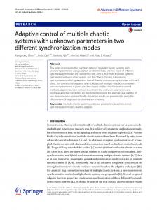
where [𝑥1 (𝑡) 𝑥2 (𝑡) 𝑥3 (𝑡)]𝑇 and [𝑥̂1 (𝑡) 𝑥̂2 (𝑡) 𝑥̂3 (𝑡)]𝑇 are the state vectors of master and slave systems, respectively. Let the different initial conditions of master and slave systems be [𝑥1 (0) = −0.5 𝑥2 (0) = −2 𝑥3 (0) = 6] and [𝑥̂1 (0) = 1 𝑥̂2 (0) = 2 𝑥̂3 (0) = −1], and let the external disturbance 𝜕(𝑡) = 0.5 sin(2.3𝑡). Figures 2(a) and 2(b) show the chaotic behaviors of the master (38) and slave (39) systems, respectively.

neurons are chosen as follows: 𝑇 (V𝜍𝜎 (𝑡)) = {

[1 + exp (−V𝜍𝜎 (𝑡) /0.5)]

− 1} (40)

for 𝜎 = 1, 2. On the other hand, the transfer functions of all output neurons are chosen as follows:

Solution. We can solve the above problem according to the following steps. Step 1. Establish the NN models for master and slave systems via back propagation algorithm, respectively. First, the NN model to approximate the master chaotic system is constructed by 4–5–3, and the transfer functions of all hidden

2

𝑇 (V𝜍𝜎 (𝑡)) = V𝜍𝜎 (𝑡) ,

for 𝜎 = 3.

(41)

After training, we can obtain the following the connection 𝜎 weights (the indices in 𝑊𝜍𝜗 state that the weight of the 𝜎th layer in the NN model represents the connection to the 𝜍th neuron from the 𝜗th source):

𝑊1 1 = [𝑊𝜍𝜗 ] = 10−3

−2.2596 1.9650 −0.0363 −0.0032 −508.2983 −548.8484 632.4534 0.0048 563.0571 790.8728 −126.7520 −0.0013 [ −15.5783 −27.7458 −63.4663 1.0173 586.7615 −331.7273 682.0762 0.4348 904.2274 −284.3785 413.0475 −4.4174 ] × [ 70.0573 −51.6754 2.1679 0.2317 807.5113 −966.2829 −831.8849 −0.2983 217.1861 −763.1395 788.9868 0.0089 ] , 52.1919 −18.8304 −51.5188 1.8090 814.8914 −164.8514 939.5783 −1.5049 −391.4165 −277.6515 −780.2455 −3.8781 ] [

90042.4610 265.5050 1364.4214 [−99246.709 772.631 −4313.1671 [ 2 𝑊2 = [𝑊𝜍𝜗 ] = 10−3 × [ [−221487.76 −1715.2506 −9271.4255 [−6724.7569 0949.6135 −624.7541 [ 93499.239 −735.4193 4088.0257

−132.9508 605.4461 ] ] −413.9966] ], −433.4421] −799.674 ]

349642.81 39165.768 −13541.566 −87345.175 56762.8100 3 ] = 10−3 × [ 702.9312 844318.23 117376.51 −667488.67 393028.9 ] . 𝑊3 = [𝑊𝜍𝜗 [82032.708 5430424.3 −402721.53 −952938.89 5075605.6 ]

Then, the net inputs of the 𝜎th (𝜎 = 1, 2, 3) layer are

(42)

+ 𝑊𝜍71 ⋅ 0 + 𝑊𝜍81 𝑥2 (𝑡 − 0.055) + 𝑊𝜍91 ⋅ 0 1 1 1 + 𝑊𝜍10 ⋅ 0 + 𝑊𝜍11 ⋅ 0 + 𝑊𝜍12 𝑥2 (𝑡 − 0.12) ,

𝜍 = 1, 2, 3, 4,

V𝜍1 (𝑡) = 𝑊𝜍11 𝑥1 (𝑡) + 𝑊𝜍21 𝑥2 (𝑡) + 𝑊𝜍31 𝑥3 (𝑡) +

𝑊𝜍41 𝑥1

(𝑡 − 0.15) +

𝑊𝜍51

⋅0+

𝑊𝜍61

⋅0

(43a)


9

V𝜍2 (𝑡) = 𝑊𝜍12 𝑇 (V11 (𝑡)) + 𝑊𝜍22 𝑇 (V21 (𝑡)) + 𝑊𝜍32 𝑇 (V31 (𝑡)) + 𝑊𝜍42 𝑇 (V41 (𝑡)) ,

+ 𝑔𝑟1 𝑊𝜍32 V31 (𝑡) + 𝑔𝑜1 𝑊𝜍42 V41 (𝑡)) (43b)

𝑑 =0

𝜍 = 1, 2, 3, 4, 5,

1

+

(𝑡)) +

𝑊𝜍43 𝑇 (V42

+ 𝑊𝜍53 𝑇 (V52 (𝑡)) ,

1

1

1

𝑐 =0 𝑙 =0 𝑘 =0 𝑚 =0 𝑛 =0

(𝑡))

2 2 2 × ℎ3𝑘 (𝑡) ℎ4𝑚 (𝑡) ℎ5𝑛 (𝑡)

𝜍 = 1, 2, 3,

1

(43c)

1

1

1

1 1 1 1 ⋅ ∑ ∑ ∑ ∑ ℎ1𝑠 (𝑡) ℎ2𝑝 (𝑡) ℎ3𝑟 (𝑡) ℎ4𝑜 (𝑡) 𝑠 =0 𝑝 =0 𝑟 =0 𝑜 =0

𝑇 (V13

(𝑡)) 𝑥1̇ (𝑡) [ ] [ ] 𝑋̇ (𝑡) = [𝑥2̇ (𝑡)] = [𝑇 (V23 (𝑡))] [ ] 3 [𝑥3̇ (𝑡)] 𝑇 (V (𝑡)) 3 [ ]

3 1 2 1 × (𝑔𝑐2 𝑊11 𝑔𝑠 𝑊11 V1 (𝑡)

(43d)

3 1 2 1 + 𝑔𝑐2 𝑊11 𝑔𝑝 𝑊12 V2 (𝑡) 3 1 2 1 + 𝑔𝑐2 𝑊11 𝑔𝑟 𝑊13 V3 (𝑡)

(the symbol V𝜍𝜎 denotes the net input of the 𝜍th neuron of the 𝜎th layer in the NN model, and the indices 𝜎 and 𝜍 shown in 𝜎 (𝜑 = 1, 2) indicate the same thing). ℎ𝜍𝜑 According to (9), the minimum and the maximum of the derivative of each transfer function shown in (40) and (41) can be obtained as follows: 1 2 = 𝑔𝜍0 = 0, 𝑔𝜍0 1 2 3 𝑔𝜍1 = 𝑔𝜍1 = 𝑔𝜍1 = 1,

3 𝑔𝜍0 = 1,

for 𝜍 = 1, 2, . . . , 𝐽𝜎 .

1

2 2 × ∑ ∑ ∑ ∑ ∑ ℎ1𝑐 (𝑡) ℎ2𝑙 (𝑡)

V𝜍3 (𝑡) = 𝑊𝜍13 𝑇 (V12 (𝑡)) + 𝑊𝜍23 𝑇 (V22 (𝑡)) 𝑊𝜍33 𝑇 (V32

1

3 = ∑ ℎ1𝑑 (𝑡) 𝑔𝑑3

3 1 2 1 + 𝑔𝑐2 𝑊11 𝑔𝑜 𝑊14 V4 (𝑡) 3 1 2 1 + 𝑔𝑙2 𝑊12 𝑔𝑠 𝑊21 V1 (𝑡) 3 1 2 1 + 𝑔𝑙2 𝑊12 𝑔𝑝 𝑊22 V2 (𝑡) 3 1 2 1 + 𝑔𝑙2 𝑊12 𝑔𝑟 𝑊23 V3 (𝑡)

(44)

3 1 2 1 + 𝑔𝑙2 𝑊12 𝑔𝑜 𝑊24 V4 (𝑡) 3 1 2 1 + 𝑔𝑘2 𝑊13 𝑔𝑠 𝑊31 V1 (𝑡)

1 1 2 To simplify the notation, we let 𝑔𝜍0 = 𝑔01 , 𝑔𝜍1 = 𝑔11 , 𝑔𝜍0 = 2 2 2 3 3 3 3 𝑔0 , 𝑔𝜍1 = 𝑔1 , 𝑔𝜍0 = 𝑔0 , and 𝑔𝜍1 = 𝑔1 . Then, based on the interpolation method, we have

3 1 2 1 + 𝑔𝑘2 𝑊13 𝑔𝑝 𝑊32 V2 (𝑡) 3 1 2 1 + 𝑔𝑘2 𝑊13 𝑔𝑟 𝑊33 V3 (𝑡)

1

5

𝑑 =0

𝜍 =1

1

5

2 3 1 2 1 + 𝑔𝑚 𝑊14 𝑔𝑠 𝑊41 V1 (𝑡)

𝑑 =0

𝜍 =1

2 3 1 2 1 + 𝑔𝑚 𝑊14 𝑔𝑝 𝑊42 V2 (𝑡)

3 1 2 1 + 𝑔𝑘2 𝑊13 𝑔𝑜 𝑊34 V4 (𝑡)

3 𝑥1̇ (𝑡) = ∑ ℎ1𝑑 (𝑡) 𝑔𝑑3 ∑ 𝑊1𝜍3 𝑇 (V𝜍2 (𝑡))

3 2 2 = ∑ ℎ1𝑑 (𝑡) 𝑔𝑑3 ∑ 𝑊1𝜍3 (ℎ𝜍0 (𝑡) 𝑔02 + ℎ𝜍1 (𝑡) 𝑔12 ) 4

×

∑ 𝑊𝜍𝜐2 𝑇 (V𝜐1 𝜐 =1

1

5

𝑑 =0

𝜍 =1

2 3 1 2 1 + 𝑔𝑚 𝑊14 𝑔𝑟 𝑊43 V3 (𝑡)

(𝑡))

2 3 1 2 1 𝑊14 𝑔𝑜 𝑊44 V4 (𝑡) + 𝑔𝑚 3 1 2 1 + 𝑔𝑛2 𝑊15 𝑔𝑠 𝑊51 V1 (𝑡)


3 1 2 1 + 𝑔𝑛2 𝑊15 𝑔𝑝 𝑊52 V2 (𝑡)

𝜐 =1

3 1 2 1 𝑔𝑟 𝑊53 V3 (𝑡) + 𝑔𝑛2 𝑊15

1 1 × ∑ 𝑊𝜍𝜐2 (ℎ𝜐0 (𝑡) 𝑔01 + ℎ𝜐1 (𝑡) 𝑔11 ) V𝜐1 (𝑡) 1

5

𝑑 =0

𝜍 =1

3 1 2 1 + 𝑔𝑛2 𝑊15 𝑔𝑜 𝑊54 V4 (𝑡)) ,


1

1

1

1 1 1 1 × ∑ ∑ ∑ ∑ ℎ1𝑠 (𝑡) ℎ2𝑝 (𝑡) ℎ3𝑟 (𝑡) ℎ4𝑜 (𝑡) 𝑠 =0 𝑝 =0 𝑟 =0 𝑜 =0

⋅ (𝑔𝑠1 𝑊𝜍12 V11 (𝑡) + 𝑔𝑝1 𝑊𝜍22 V21 (𝑡)

1

5

𝑒 =0

𝜍 =1

1

5

𝑒 =0

𝜍 =1

3 𝑥2̇ (𝑡) = ∑ ℎ2𝑒 (𝑡) 𝑔𝑒3 ∑ 𝑊2𝜍3 𝑇 (V𝜍2 (𝑡))

3 2 2 = ∑ ℎ2𝑒 (𝑡) 𝑔𝑒3 ∑ 𝑊2𝜍3 (ℎ𝜍0 (𝑡) 𝑔02 + ℎ𝜍1 (𝑡) 𝑔12 )

10

Abstract and Applied Analysis 2 3 1 2 1 𝑊24 𝑔𝑜 𝑊44 V4 (𝑡) + 𝑔𝑚

4

× ∑ 𝑊𝜍𝜐2 𝑇 (V𝜐1 (𝑡)) 1

5

3 1 2 1 + 𝑔𝑛2 𝑊25 𝑔𝑠 𝑊51 V1 (𝑡)

𝑒 =0

𝜍 =1

3 1 2 1 + 𝑔𝑛2 𝑊25 𝑔𝑝 𝑊52 V2 (𝑡)

𝜐 =1

3 2 2 = ∑ ℎ2𝑒 (𝑡) 𝑔𝑒3 ∑ 𝑊2𝜍3 (ℎ𝜍0 (𝑡) 𝑔02 + ℎ𝜍1 (𝑡) 𝑔12 )

×

4

∑ 𝑊𝜍𝜐2 𝜐 =1

1 (ℎ𝜐0

(𝑡) 𝑔01

+

1 ℎ𝜐1

(𝑡) 𝑔11 ) V𝜐1

3 1 2 1 + 𝑔𝑛2 𝑊25 𝑔𝑟 𝑊53 V3 (𝑡)

(𝑡)

3 1 2 1 𝑔𝑜 𝑊54 V4 (𝑡)) , + 𝑔𝑛2 𝑊25

5

1

3 2 2 = ∑ ℎ2𝑒 (𝑡) 𝑔𝑒3 ∑ 𝑊2𝜍3 (ℎ𝜍0 (𝑡) 𝑔02 + ℎ𝜍1 (𝑡) 𝑔12 ) 𝑒 =0

𝜍 =1

1

1

1

1

1 1 1 1 × ∑ ∑ ∑ ∑ ℎ1𝑠 (𝑡) ℎ2𝑝 (𝑡) ℎ3𝑟 (𝑡) ℎ4𝑜 (𝑡)

⋅

(𝑡) +

𝑔𝑝1 𝑊𝜍22 V21

(𝑡)

=

3 ∑ ℎ2𝑒 𝑒 =0

⋅

1

1

1

5

𝑓= 0

𝜍 =1

𝜐 =1

1 1 1 1 1 2 (𝑡) 𝑔𝑒3 ∑ ∑ ∑ ∑ ∑ ℎ1𝑐 𝑐 =0 𝑙 =0 𝑘 =0 𝑚 =0 𝑛 =0

1

𝜍 =1

4

2 (𝑡) ℎ2𝑙

2 (𝑡) ℎ3𝑘

(𝑡)

2 2 × ℎ4𝑚 (𝑡) ℎ5𝑛 (𝑡) 1

𝑓= 0

× ∑ 𝑊𝜍𝜐2 𝑇 (V𝜐1 (𝑡))

+ 𝑔𝑟1 𝑊𝜍32 V31 (𝑡) + 𝑔𝑜1 𝑊𝜍42 V41 (𝑡)) 1

5

3 2 2 = ∑ ℎ3𝑓 (𝑡) 𝑔𝑓3 ∑ 𝑊3𝜍3 (ℎ𝜍0 (𝑡) 𝑔02 + ℎ𝜍1 (𝑡) 𝑔12 )

𝑠 =0 𝑝 =0 𝑟 =0 𝑜 =0

(𝑔𝑠1 𝑊𝜍12 V11

1

3 𝑥3̇ (𝑡) = ∑ ℎ3𝑓 (𝑡) 𝑔𝑓3 ∑ 𝑊3𝜍3 𝑇 (V𝜍2 (𝑡))

1

5

𝑓= 0

𝜍 =1

3 2 2 = ∑ ℎ3𝑓 (𝑡) 𝑔𝑓3 ∑ 𝑊3𝜍3 (ℎ𝜍0 (𝑡) 𝑔02 + ℎ𝜍1 (𝑡) 𝑔12 ) 4

1 1 × ∑ 𝑊𝜍𝜐2 (ℎ𝜐0 (𝑡) 𝑔01 + ℎ𝜐1 (𝑡) 𝑔11 ) V𝜐1 (𝑡) 𝜐 =1

1 ∑ ∑ ∑ ∑ ℎ1𝑠 𝑠 =0 𝑝 =0 𝑟 =0 𝑜 =0

1 (𝑡) ℎ2𝑝

1 (𝑡) ℎ3𝑟

1 (𝑡) ℎ4𝑜

(𝑡)

3 1 2 1 × (𝑔𝑐2 𝑊21 𝑔𝑠 𝑊11 V1 (𝑡)

1

5

𝑓= 0

𝜍 =1

3 2 2 = ∑ ℎ3𝑓 (𝑡) 𝑔𝑓3 ∑ 𝑊3𝜍3 (ℎ𝜍0 (𝑡) 𝑔02 + ℎ𝜍1 (𝑡) 𝑔12 ) 1

3 1 2 1 𝑔𝑝 𝑊12 V2 (𝑡) + 𝑔𝑐2 𝑊21 3 1 2 1 𝑔𝑟 𝑊13 V3 (𝑡) + 𝑔𝑐2 𝑊21

3 1 2 1 + 𝑔𝑙2 𝑊22 𝑔𝑝 𝑊22 V2 (𝑡)

+

3 1 2 1 𝑔𝑟 𝑊23 V3 𝑔𝑙2 𝑊22

+

3 1 2 1 𝑔𝑙2 𝑊22 𝑔𝑜 𝑊24 V4

(𝑡)

+

3 1 2 1 𝑔𝑘2 𝑊23 𝑔𝑠 𝑊31 V1

(𝑡)

(𝑡)

3 1 2 1 + 𝑔𝑘2 𝑊23 𝑔𝑝 𝑊32 V2 (𝑡) 3 1 2 1 + 𝑔𝑘2 𝑊23 𝑔𝑟 𝑊33 V3 (𝑡) 3 1 2 1 + 𝑔𝑘2 𝑊23 𝑔𝑜 𝑊34 V4 (𝑡) 2 3 1 2 1 𝑊24 𝑔𝑠 𝑊41 V1 (𝑡) + 𝑔𝑚

1

1

𝑠 =0 𝑝 =0 𝑟 =0 𝑜 =0

⋅ (𝑔𝑠1 𝑊𝜍12 V11 (𝑡) + 𝑔𝑝1 𝑊𝜍22 V21 (𝑡) + 𝑔𝑟1 𝑊𝜍32 V31 (𝑡) + 𝑔𝑜1 𝑊𝜍42 V41 (𝑡))

3 1 2 1 + 𝑔𝑐2 𝑊21 𝑔𝑜 𝑊14 V4 (𝑡) 3 1 2 1 + 𝑔𝑙2 𝑊22 𝑔𝑠 𝑊21 V1 (𝑡)

1

1 1 1 1 × ∑ ∑ ∑ ∑ ℎ1𝑠 (𝑡) ℎ2𝑝 (𝑡) ℎ3𝑟 (𝑡) ℎ4𝑜 (𝑡)

1

1

1

1

1

1

3 2 2 2 = ∑ ℎ3𝑓 (𝑡) 𝑔𝑓3 ∑ ∑ ∑ ∑ ∑ ℎ1𝑐 (𝑡) ℎ2𝑙 (𝑡) ℎ3𝑘 (𝑡) 𝑐 =0 𝑙 =0 𝑘 =0 𝑚 =0 𝑛 =0

𝑓= 0

2 2 × ℎ4𝑚 (𝑡) ℎ5𝑛 (𝑡) 2

2

2

2

1 1 1 1 ⋅ ∑ ∑ ∑ ∑ ℎ1𝑠 (𝑡) ℎ2𝑝 (𝑡) ℎ3𝑟 (𝑡) ℎ4𝑜 (𝑡) 𝑠 =1 𝑝 =1 𝑟 =1 𝑜 =1

3 1 2 1 × (𝑔𝑐2 𝑊31 𝑔𝑠 𝑊11 V1 (𝑡) 3 1 2 1 + 𝑔𝑐2 𝑊31 𝑔𝑝 𝑊12 V2 (𝑡) 3 1 2 1 + 𝑔𝑐2 𝑊31 𝑔𝑟 𝑊13 V3 (𝑡) 3 1 2 1 𝑔𝑜 𝑊14 V4 (𝑡) + 𝑔𝑐2 𝑊31 3 1 2 1 𝑔𝑠 𝑊21 V1 (𝑡) + 𝑔𝑙2 𝑊32

2 3 1 2 1 + 𝑔𝑚 𝑊24 𝑔𝑝 𝑊42 V2 (𝑡)

3 1 2 1 𝑔𝑝 𝑊22 V2 (𝑡) + 𝑔𝑙2 𝑊32

2 3 1 2 1 + 𝑔𝑚 𝑊24 𝑔𝑟 𝑊43 V3 (𝑡)

3 1 2 1 + 𝑔𝑙2 𝑊32 𝑔𝑟 𝑊23 V3 (𝑡)


11

3 1 2 1 + 𝑔𝑙2 𝑊32 𝑔𝑜 𝑊24 V4 (𝑡)

Based on (10), let

3 1 2 1 + 𝑔𝑘2 𝑊33 𝑔𝑠 𝑊31 V1 (𝑡)

+

3 1 2 1 𝑔𝑘2 𝑊33 𝑔𝑝 𝑊32 V2

𝑔𝑠1 0 0 [ 0 𝑔𝑝1 0 𝐺1 = [ [ 0 0 𝑔1 𝑟 [0 0 0

(𝑡)

3 1 2 1 + 𝑔𝑘2 𝑊33 𝑔𝑟 𝑊33 V3 (𝑡) 2 3 1 2 1 + 𝑔𝑘 𝑊33 𝑔𝑜 𝑊34 V4 (𝑡)

+

2 3 1 2 1 𝑔𝑚 𝑊34 𝑔𝑠 𝑊41 V1

(𝑡)

2 𝐺33

2 3 1 2 1 + 𝑔𝑚 𝑊34 𝑔𝑝 𝑊42 V2 (𝑡) 2 3 1 2 1 + 𝑔𝑚 𝑊34 𝑔𝑟 𝑊43 V3 (𝑡)

+

2 3 1 2 1 𝑔𝑚 𝑊34 𝑔𝑜 𝑊44 V4

(𝑡)

R = 1, 2, 3; ℵ = 1, 2 . . . , 12. (45)

1

1

1

0 0] ] 0] ], 0] 𝑔𝑛2 ]

𝐸𝑑𝑒𝑓𝑐𝑙𝑘𝑚𝑛𝑠𝑝𝑟𝑜𝑞 ≡ 𝐺3 𝑊3 𝐺2 𝑊2 𝐺1 𝑊1 = [ΥRℵ ]3×12 ,

3 1 2 1 𝑔𝑜 𝑊54 V4 (𝑡)) . + 𝑔𝑛2 𝑊35

1

0 0 0 2 𝑔𝑚 0

(46)

Then,

3 1 2 1 + 𝑔𝑛2 𝑊35 𝑔𝑟 𝑊53 V3 (𝑡)

1

0 0 𝑔𝑘2 0 0

𝑔3 0 0 [ 0𝑑 𝑔3 0 ] 𝐺 =[ ]. 𝑒 0 0 𝑔𝑓3 [ ]

3 1 2 1 + 𝑔𝑛2 𝑊35 𝑔𝑝 𝑊52 V2 (𝑡)

1

0 𝑔𝑙2 0 0 0

3

3 1 2 1 + 𝑔𝑛2 𝑊35 𝑔𝑠 𝑊51 V1 (𝑡)

1

𝑔𝑐2 [0 [ =[ [0 [0 [0

0 0] ], 0] 𝑔𝑜1 ]

1

1

1

1

(47)

Plugging (43a)–(43c) into (45) leads to 1

2 2 2 2 2 2 2 2 𝑋̇ (𝑡) = ∑ ∑ ∑ ∑ ∑ ∑ ∑ ∑ ∑ ∑ ∑ ∑ ℎ1𝑑 (𝑡) ℎ2𝑒 (𝑡) ℎ3𝑓 (𝑡) ℎ1𝑐 (𝑡) ℎ2𝑙 (𝑡) ℎ3𝑘 (𝑡) ℎ4𝑚 (𝑡) ℎ5𝑛 (𝑡) 𝑑=0 𝑒=0 𝑓=0 𝑐=0 𝑙=0 𝑘=0 𝑚=0 𝑛=0 𝑠=0 𝑝=0 𝑟=0 𝑜=0

(48)

1 1 1 1 ⋅ ℎ1𝑠 (𝑡) ℎ2𝑝 (𝑡) ℎ3𝑟 (𝑡) ℎ4𝑜 (𝑡) {𝐴 𝑑𝑒𝑓𝑐𝑙𝑘𝑚𝑛𝑠𝑝𝑟𝑜 𝑋 (𝑡) + 𝐴𝑑𝑒𝑓𝑐𝑙𝑘𝑚𝑛𝑠𝑝𝑟𝑜1 𝑋 (𝑡 − 0.15)

+ 𝐴𝑑𝑒𝑓𝑐𝑙𝑘𝑚𝑛𝑠𝑝𝑟𝑜2 𝑋 (𝑡 − 0.055) + 𝐴𝑑𝑒𝑓𝑐𝑙𝑘𝑚𝑛𝑠𝑝𝑟𝑜3 𝑋 (𝑡 − 0.12)} ,

where

Next, by renumbering the matrices shown in (48), the NN model of master system can be rewritten as the following LDI state-space representation:

Υ1 1 Υ1 2 Υ1 3 𝐴 𝑑𝑒𝑓𝑐𝑙𝑘𝑚𝑛𝑠𝑝𝑟𝑜 = [Υ2 1 Υ2 2 Υ2 3 ] , [Υ3 1 Υ3 2 Υ3 3 ] 𝐴𝑑𝑒𝑓𝑐𝑙𝑘𝑚𝑛𝑠𝑝𝑟𝑜1

Υ1 4 Υ1 5 Υ1 6 = [Υ2 4 Υ2 5 Υ2 6 ] , [Υ3 4 Υ3 5 Υ3 6 ]

𝑖 =1

𝑘 =1

(50)

𝐴 1 = 𝐴 000000000000 , . . . , 𝐴 4065 = 𝐴 111111111110 , 𝐴 4096 = 𝐴 111111111111 ,

Υ1 10 Υ1 11 Υ1 12 = [Υ2 10 Υ2 11 Υ2 12 ] , [Υ3 10 Υ3 11 Υ3 12 ] 𝑇

𝑋 (𝑡) = [𝑥1 (𝑡) 𝑥2 (𝑡) 𝑥3 (𝑡)] , 𝑇

𝑋 (𝑡 − 0.15) = [𝑥1 (𝑡 − 0.15) 0 0] , 𝑇

𝑋 (𝑡 − 0.055) = [0 𝑥2 (𝑡 − 0.055) 0] , 𝑇

3

where 𝜏1 = 0.15, 𝜏2 = 0.055, 𝜏3 = 0.12,

Υ1 7 Υ1 8 Υ1 9 𝐴𝑑𝑒𝑓𝑐𝑙𝑘𝑚𝑛𝑠𝑝𝑟𝑜2 = [Υ2 7 Υ2 8 Υ2 9 ] , [Υ3 7 Υ3 8 Υ3 9 ] 𝐴𝑑𝑒𝑓𝑐𝑙𝑘𝑚𝑛𝑠𝑝𝑟𝑜3

4096

𝑋̇ (𝑡) = ∑ ℎ𝑖 (𝑡) {𝐴 𝑖 𝑋 (𝑡) + ∑ 𝐴𝑖𝑘 𝑋 (𝑡 − 𝜏𝑘 )} ,

𝑋 (𝑡 − 0.12) = [0 0 𝑥3 (𝑡 − 0.12)] .

(49)

𝐴1 1 = 𝐴 000000000000 1 , . . . , 𝐴4095 1 = 𝐴 111111111110 1 , 𝐴4096 1 = 𝐴 111111111111 1 , 𝐴1 2 = 𝐴 000000000000 2 , . . . , 𝐴4095 2 = 𝐴 111111111110 2 , 𝐴4096 2 = 𝐴 111111111111 2 , 𝐴1 3 = 𝐴 000000000000 3 , . . . , 𝐴4095 3 = 𝐴 111111111110 3 , 𝐴4096 3 = 𝐴 111111111111 3 .

(51)

12


Similarly, the connection weights of the NN model for the slave system are obtained as follows: ̂1 = [𝑊 ̂1 ] = 10−3 𝑊 𝜍𝜗 133.4435

−62.4012 × [−136.5871 [ 46.5562

−0079.5049 −17.6211 3.3882 −225.1168 −64.0209 −954.1527 −3.4193 480.1857 754.7737 707.4367 −2.159 53.2513 −4.9754 0.4651 −383.4523 −999.858 275.4848 −0.25 −190.4024 655.3 295.4735 −0.2102] 80.423 17.6424 −3.432 −335.9 451.561 −121.296 3.4809 −897.175 −102.7268 13.5665 2.1915 , 10.9547 24.1296 −1.6127 863.1865 −201.0341 183.5383 0.7656 896.0093 768.9494 −847.9542 0.5831 ]

21614.815 [−2215.2823 [ ̂2 = [W ̂ 2 ] = 10−3 × [ −989.3919 𝑊 𝜍𝜗 [ [ 128543.46 [−24482.498

1817.1715 17964.295 −1655.6057 0.641.7697 −2.146.7808 121.167 ] ] −1389.4418 −1046.1459 −410.0032 ] ], −5108.3101 127475.58 2979.3142 ] 1165.7441 −27137.819 −2515.8115]

−215587.43 1177534.5 123780.4 18638.275 240168.12 ̂3 ] = 10−3 × [ 294714.01 312655.73 −198923.25 −55013.034 −330253.83] . ̂3 = [𝑊 𝑊 𝜍𝜗 2000786 −48419.674 1579125.9 ] [−1607287.8 4247988

Step 2. The procedures of constructing the NN model for the slave system are similar to those for the master system, and then we have the NN model of the slave system: 4096

3

𝑗 =1

𝑘 =1

̂ 𝑋 ̂ (𝑡) + ∑ 𝐴 ̂ ̂̇ (𝑡) = ∑ ̂ℎ𝑗 (𝑡) {𝐴 ̂𝑗 𝑋 𝑋 𝑗𝑘 (𝑡 − 𝜏𝑘 )} + 𝐵𝑈 (𝑡) (53) with 𝜏1 = 0.15, 𝜏2 = 0.055, 𝜏3 = 0.12, and B is a identity ̂̇ for original systems ̇ and 𝑋(𝑡) matrix. The responses of 𝑋(𝑡) and NN models are shown in Figures 3(a) and 3(b). Step 3. To synchronize the master and slave systems, a fuzzy controller is synthesized as follows: Control Rule 1: IF 𝑒1 (𝑡) is 𝑀1 ,

THEN 𝑈 (𝑡) = −𝐾1 𝐸 (𝑡) ,

Control Rule 2: IF 𝑒1 (𝑡) is 𝑀2 ,

THEN 𝑈 (𝑡) = −𝐾2 𝐸 (𝑡) , (54)

where 𝑀1 and 𝑀2 are the membership functions for each 𝑒1 (see Figure 4): 1, 𝑒1 ≥ 30, { { { 𝑒1 𝑀1 (𝑒1 ) = { , −30 < 𝑒1 < 30, { { 30 𝑒1 ≤ −30, {1,

(55a)

𝑀2 (𝑒1 ) = 1 − 𝑀1 (𝑒1 ) .

(55b)

∑2𝑙=1 𝑤𝑙 (𝑡) 𝐾𝑙 𝐸 (𝑡) ∑2𝑙=1

𝑤𝑙 (𝑡)

2

= − ∑ ℎ𝑙 (𝑡) 𝐾𝑙𝑙 𝐸 (𝑡) 𝑙 =1

with 𝑤𝑙 (𝑡) ≡ 𝑀𝑙 (𝑒1 (𝑡)), ℎ𝑙 (𝑡) ≡ 𝑤𝑙 (𝑡)/(∑2𝑙=1 𝑤𝑙 (𝑡)).

According to (21), the dynamics of the error system is obtained as follows: 4096 2

𝐸̇ (𝑡) = ∑ ∑ ℎ𝑖 (𝑡) ℎ𝑙 (𝑡) 𝑖 =1 𝑙 =1

3

× {𝐷𝑖𝑙 𝐸 (𝑡) + ∑ 𝐴𝑖𝑘 𝐸 (𝑡 − 𝜏𝑘 )}

(57)

𝑘 =1

+ 𝜕 (𝑡) + Φ (𝑡) , 3 ̂ ̂ where 𝐷𝑖𝑙 ≡ 𝐴 𝑖 −𝐵𝐾𝑙 , Γ̂ ≡ 𝑓(𝑋(𝑡))+∑ 𝑘 =1 𝐻𝑘 (𝑋(𝑡−𝜏𝑘 ))+𝑈(𝑡) 2 with 𝑈(𝑡) = − ∑𝑙 =1 ℎ𝑙 (𝑡)𝐾𝑙 𝐸(𝑡), 3

Γ ≡ 𝑓 (𝑋 (𝑡)) + ∑ 𝐻𝑘 (𝑋 (𝑡 − 𝜏𝑘 )) , 𝑘=1

4096 2

Φ (𝑡) ≡ Γ̂ − Γ− { ∑ ∑ℎ𝑖 (𝑡) ℎ𝑙 (𝑡) [𝐷𝑖𝑙 𝐸 (𝑡)

(58)

𝑖=1 𝑙=1 3

+ ∑ 𝐴𝑖𝑘 𝐸 (𝑡 − 𝜏𝑘 )]} . 𝑘=1

According to (20), we have the overall fuzzy controller: 𝑈 (𝑡) = −

(52)

(56)

Step 4. Based on (42), (48)–(57), the LMI in (34a) and (34b) can be solved via MATLAB LMI Toolbox. In accordance with Remark 1, the specified structured bounding matrices 4600 0 0 100 𝑌 and 𝜅𝑖𝑙 are set to be 𝑌 = [ 0 4600 0 ], 𝜅𝑖𝑙 = [ 0 1 0 ]. 0 0 4600 001 Based on Corollary 11, the positive constant 𝑐 is minimized by the mincx function of MATLAB LMI Toolbox: 𝑐min = 5.3341 × 10−15 , and then we have the minimum disturbance attenuation level 𝛾min = 1.0329 × 10−7 . Step 5. The common solutions 𝑃, 𝐹1 , 𝐹2 , 𝜓1 , 𝜓2 , and 𝜓3 of the stability conditions (32b) and (32c) can be obtained with

.

x1


13

200

200

0

0

−200

−200 0

1

2

3

4

5 6 Time (s)

7

8

9

10

0

.

x2

200

0

0 1

2

3

4

5 6 Time (s)

7

8

9

10

−200

0

Original Model

.

4

5

6

7

8

9

10

1

2

3

4

5 6 Time (s)

7

8

9

10

3

4

5 6 Time (s)

7

8

9

10

Original Model 400 200 0 −200

3

x3

400 200 0 −200

3

Original Model

200

0

2

Time (s)

Original Model

−200

1

0

1

2

3

4

5 6 Time (s)

7

8

9

10

Original Model

0

1

2

Original Model (a)

(b)

̂̇ for original system and NN model. ̇ for original system and NN model. (b) The responses of 𝑋(𝑡) Figure 3: (a) The responses of 𝑋(𝑡)

the best value 𝑡 min of LMI Solver (MATLAB) of −1.135048× 10−8 : 4001.1183 −268.3795 813.795 𝑃 = 104 × [−268.3795 2206.7761 778.8835 ] , [ 813.795 778.8835 3191.7162] 0.1113 0.0257 −0.0346 𝐹1 = 10−3 × [ 0.0258 0.2094 −0.0576] , [−0.0347 −0.0578 0.1515 ]

(59)

6. Conclusion

0.1113 0.0258 −0.0347 𝐹2 = 10−3 × [ 0.0258 0.2094 −0.0576] . [−0.0347 −0.0576 0.1515 ] Furthermore, the resulting controller gains are 4103.0292 −1.3653 0.8911 𝐾1 = [ 1.3645 4103.0282 2.2966 ] , [ −0.8907 −2.2952 4103.0288] 4103.0292 −0.624 −0.6759 𝐾2 = [ 0.6233 4103.0282 1.7095 ] , −1.7081 4103.0288] [ 0.6763 0.6228 0.0000 0.0000 𝜓1 = 𝜓2 = 𝜓3 = [0.0000 0.6228 0.0001] . [0.0000 0.0001 0.6228]

Figure 5 displays the state responses of both master and slave systems. The chaotic behaviors of the master and slave systems are shown in Figure 6. Moreover, Figure 7 illustrates the synchronization errors (𝑒1 , 𝑒2 , and 𝑒3 ) which converge to zero. Furthermore, the assumption of ‖Φ(𝑡)‖ ≤ 2 ‖ ∑4096 𝑖 =1 ∑𝑙 =1 ℎ𝑖 (𝑡)ℎ𝑙 (𝑡)Δ𝑌𝑖𝑙 𝐸(𝑡)‖ is satisfied from the illustration shown in Figure 8.

(60)

In this study, an effective approach is proposed to realize the exponential synchronization of multiple time-delay chaotic (MTDC) systems, and the optimal 𝐻∞ performance is achieved at the same time. First, we employed a neural network (NN) model to approximate the MTDC system. A linear differential inclusion (LDI) state-space representation is then established for the dynamics of the NN model. Next, a delay-dependent stability criterion derived in terms of Lyapunov’s direct method is presented to guarantee that the slave system can exponentially synchronize with the master system. Subsequently, the stability condition of this criterion is reformulated into a linear matrix inequality (LMI). Based on the Lyapunov stability theory and LMI approach, a fuzzy controller is synthesized to realize the exponential 𝐻∞ synchronization of the chaotic master-slave systems and reduce the 𝐻∞ -norm from disturbance to synchronization error at the lowest level. Finally, simulation results demonstrate that

14

Abstract and Applied Analysis 1

50

0.9

40

0.7

30

0.6

20

𝑥3 (𝑡)

Grade

0.8

0.5 0.4

10 0

0.3

−10 20 10

0.2 0.1 0 10 Time (s)

20

30

40

50

(𝑡) 𝑥2

0 −50 −40 −30 −20 −10

0 −10 −20

𝑀1 𝑀2

0

−5

−20 −15 −10

5

10

15

20

𝑥1 (𝑡) Master Slave

Figure 4: Membership functions of the fuzzy controller.

Figure 6: The chaotic behaviors of the master and the slave systems.

0

0.02 0.04 0.06 0.08 0.1 0.12 0.14 0.16 0.18 Time (s)

0.2

10 0 −10 −20

𝑒1

𝑥1 ̂1 𝑥

0

0.02 0.04 0.06 0.08 0.1 0.12 0.14 0.16 0.18 Time (s)

0

0.05

0.1

0.15

0.2

0.25

0.3

0.35

0.4

0.45

0.5

0.3

0.35

0.4

0.45

0.5

0.3

0.35

0.4

0.45

0.5

𝑒1

0.2

𝑒2

𝑥2 ̂2 𝑥 15 10 5 0 −5

4 2 0 −2 −4

Time (s)

10 5 0 −5 −10

0

0.05

0.1

0.15

0.2

0.25 Time (s)

𝑒2 0

0.02 0.04 0.06 0.08 0.1 0.12 0.14 0.16 0.18 Time (s)

0.2

𝑥3 ̂3 𝑥

𝑒3

5 0 −5 −10 −15

10 0 −10 0

0.05

0.1

0.15

0.2

0.25 Time (s)

Figure 5: State responses of both master and slave systems. 𝑒3

Figure 7: State responses of the error system. ∞

the exponential 𝐻 synchronization of MTDC systems can be achieved by the designed fuzzy controller.

Appendix Proof of Theorem 5 Let the Lyapunov function for the error system (21) be defined as

𝑚

𝑉 (𝑡) = ∑ 𝐸𝑇 (𝑡) 𝜏𝑘 𝑃𝐸 (𝑡) 𝑘 =1

𝑚

𝜏𝑘

(A.1) 𝑇

+ ∑ ∫ 𝐸 (𝑡 − 𝜋) 𝜓𝑘 𝐸 (𝑡 − 𝜋) 𝑑𝜋, 𝑘 =1 0


15 ×104 4

200

180

3.5

160

3

140 120

2.5

100 2

80 60

1.5

40

1

20 0

0.5 0

0

0

0.02

0.02 0.04 0.06 0.08 0.1 0.12 0.14 0.16 0.18 Time (s) 0.04

0.06

0.08

0.1 0.12 Time (s) 4096

0.14

0.16

0.18

0.2 0.2

2

Figure 8: Plots of ‖Φ(𝑡)‖ (blue line) and ‖ ∑𝑖 =1 ∑𝑙 =1 ℎ𝑙 (𝑡)ℎ𝑙 (𝑡)Δ𝑌𝑖𝑙 𝐸(𝑡)‖ (red line).

where the weighting matrices 𝑃 = 𝑃𝑇 > 0 and 𝜓𝑘 = 𝜓𝑘𝑇 > 0. We then evaluate the time derivative of 𝑉(𝑡) on the trajectories of (21) to obtain

𝑚

𝜙

𝜌

= ∑ ∑ ∑ ℎ𝑖 (𝑡) ℎ𝑙 (𝑡) 𝐸𝑇 (𝑡) 𝑘 =1 𝑖 =1 𝑙 =1

× [𝜏𝑘 𝐷𝑖𝑙𝑇 𝑃 + 𝜏𝑘 𝑃𝐷𝑖𝑙 + 𝜓𝑘 ] 𝐸 (𝑡) 𝜙

𝑚

𝑚

̇𝑇

𝑚

𝑇

+ ∑ ∑ ∑ ℎ𝑖 (𝑡) [𝐸𝑇 (𝑡 − 𝜏𝑑 ) 𝜏𝑘 𝐴𝑖𝑑 𝑃𝐸 (𝑡)

𝑉̇ (𝑡) = ∑ 𝜏𝑘 [𝐸 (𝑡) 𝑃𝐸 (𝑡) + 𝐸 (𝑡) 𝑃𝐸̇ (𝑡)] 𝑇

𝑘 =1 𝑖 =1 𝑑 =1

+ 𝐸𝑇 (𝑡) 𝜏𝑘 𝑃𝐴𝑖𝑑 𝐸 (𝑡 − 𝜏𝑑 )]

𝑘 =1

𝑚

+ ∑ [𝐸𝑇 (𝑡) 𝜓𝑘 𝐸 (𝑡) − 𝐸𝑇 (𝑡 − 𝜏𝑘 ) 𝜓𝑘 𝐸 (𝑡 − 𝜏𝑘 )] 𝑘 =1

𝑘 =1

𝜙

𝑚

+ Φ𝑇 (𝑡) 𝜏𝑘 𝑃𝐸 (𝑡) + 𝐸𝑇 (𝑡) 𝜏𝑘 𝑃Φ (𝑡)]

𝜌

= ∑ 𝜏𝑘 { ∑ ∑ ℎ𝑖 (𝑡) ℎ𝑙 (𝑡)

𝑚

𝑖 =1 𝑙 =1

𝑘 =1

− ∑ [𝐸𝑇 (𝑡 − 𝜏𝑘 ) 𝜓𝑘 𝐸 (𝑡 − 𝜏𝑘 )] .

𝑚

× [𝐷𝑖𝑙 𝐸 (𝑡) + ∑ 𝐴𝑖𝑑 𝐸 (𝑡 − 𝜏𝑑 )] 𝑑 =1

𝑘 =1

(A.2)

Based on Lemma 4 and (A.2), we have

𝑇

+ 𝜕 (𝑡) + Φ (𝑡) } 𝑃𝐸 (𝑡) 𝑚

𝑚

+ ∑ [𝜕𝑇 (𝑡) 𝜏𝑘 𝑃𝐸 (𝑡) + 𝐸𝑇 (𝑡) 𝜏𝑘 𝑃𝜕 (𝑡)

𝑚

𝜙

𝜌

𝑉̇ (𝑡) ≤ ∑ ∑ ∑ ℎ𝑖 (𝑡) ℎ𝑙 (𝑡) 𝐸𝑇 (𝑡) 𝑘 =1 𝑖 =1 𝑙 =1

× [𝜏𝑘 𝐷𝑖𝑙𝑇 𝑃 + 𝜏𝑘 𝑃𝐷𝑖𝑙 + 𝜓𝑘 ] 𝐸 (𝑡)

𝑇

+ ∑ 𝜏𝑘 𝐸 (𝑡) 𝑃 𝑘 =1

𝑚

𝜙

𝜌

× { ∑ ∑ ℎ𝑖 (𝑡) ℎ𝑙 (𝑡) [𝐷𝑖𝑙 𝐸 (𝑡)

𝜙

𝑚

𝑇

+ ∑ ∑ ∑ ℎ𝑖 (𝑡) [𝑎𝐸𝑇 (𝑡 − 𝜏𝑑 ) 𝐴𝑖𝑑 𝐴𝑖𝑑 𝐸 (𝑡 − 𝜏𝑑 ) 𝑘 =1 𝑖 =1 𝑑 =1

𝑖 =1 𝑙 =1

+ 𝑎−1 𝐸𝑇 (𝑡) 𝜏𝑘2 𝑃2 𝐸 (𝑡) ]

𝑚

+ ∑ 𝐴𝑖𝑑 𝐸 (𝑡 − 𝜏𝑑 ) 𝑑 =1

𝑚

+ ∑ [𝑐𝜕𝑇 (𝑡) 𝜕 (𝑡) + 𝑐−1 𝐸𝑇 (𝑡) 𝜏𝑘2 𝑃2 𝐸 (𝑡) 𝑘 =1

+ 𝑛Φ𝑇 (𝑡) Φ (𝑡) + 𝑛−1 𝐸𝑇 (𝑡) 𝜏𝑘2 𝑃2 𝐸 (𝑡)]

+ 𝜕 (𝑡) + Φ (𝑡) ]} 𝑚

𝑚

+ ∑ [𝐸𝑇 (𝑡) 𝜓𝑘 𝐸 (𝑡) − 𝐸𝑇 (𝑡 − 𝜏𝑘 ) 𝜓𝑘 𝐸 (𝑡 − 𝜏𝑘 )] 𝑘 =1

− ∑ [𝐸𝑇 (𝑡 − 𝜏𝑘 ) 𝜓𝑘 𝐸 (𝑡 − 𝜏𝑘 )] 𝑘 =1

(A.3)

16

Abstract and Applied Analysis 𝜙

𝑚

𝜌

𝜙

𝑚

≤ ∑ ∑ ∑ ℎ𝑖 (𝑡) ℎ𝑙 (𝑡) 𝐸𝑇 (𝑡)

𝑇

+ ∑ ∑ ℎ𝑖 (𝑡) 𝐸𝑇 (𝑡 − 𝜏𝑘 ) [𝑚𝑎𝐴𝑖𝑘 𝐴𝑖𝑘 − 𝜓𝑘 ]

𝑘 =1 𝑖 =1 𝑙 =1

𝑘 =1 𝑖 =1

× 𝐸 (𝑡 − 𝜏𝑘 ) + 𝑐𝑚𝜕𝑇 (𝑡) 𝜕 (𝑡) − 𝛾2 𝜕𝑇 (𝑡) 𝜕 (𝑡) (A.6a)

× [𝜏𝑘 𝐷𝑖𝑙𝑇 𝑃 + 𝜏𝑘 𝑃𝐷𝑖𝑙 + 𝜓𝑘 ] 𝐸 (𝑡) 𝜙

𝑚

𝑚

𝑇

+ ∑ ∑ ∑ ℎ𝑖 (𝑡) [𝑎𝐸𝑇 (𝑡 − 𝜏𝑑 ) 𝐴𝑖𝑑 𝐴𝑖𝑑 𝐸 (𝑡 − 𝜏𝑑 ) 𝑘 =1 𝑖 =1 𝑑 =1

𝜙

𝜌

= ∑ ∑ ℎ𝑖 (𝑡) ℎ𝑙 (𝑡) 𝐸𝑇 (𝑡) 𝑖 =1 𝑙 =1

+ 𝑎−1 𝐸𝑇 (𝑡) 𝜏𝑘2 𝑃2 𝐸 (𝑡) ]

𝑚

𝑚

𝑘 =1

𝑘 =1

× [ ∑ 𝜏𝑘 𝐷𝑖𝑙𝑇 𝑃 + ∑ 𝜏𝑘 𝑃𝐷𝑖𝑙

𝑚

+ ∑ [𝑐𝜕𝑇 (𝑡) 𝜕 (𝑡) + 𝑐−1 𝐸𝑇 (𝑡) 𝜏𝑘2 𝑃2 𝐸 (𝑡)

𝑚

𝑘 =1

+ 𝑛𝐸𝑇 (𝑡) 𝑌𝑇𝑌𝐸 (𝑡)

+ ∑ 𝜏𝑘2 𝑃2 (𝑐−1 + 𝑛−1 + 𝑚𝑎−1 )

(by (26))

𝑘 =1 𝑚

+ 𝑛−1 𝐸𝑇 (𝑡) 𝜏𝑘2 𝑃2 𝐸 (𝑡)]

+ ∑ 𝜓𝑘 + 𝑛𝑚𝑌𝑇 𝑌 + 𝐼] 𝐸 (𝑡) 𝑘 =1

𝑚

𝑇

− ∑ [𝐸 (𝑡 − 𝜏𝑘 ) 𝜓𝑘 𝐸 (𝑡 − 𝜏𝑘 )]

𝜙

𝑚

+ ∑ ∑ ℎ𝑖 (𝑡) 𝐸𝑇 (𝑡 − 𝜏𝑘 )

𝑘 =1

𝑘 =1 𝑖 =1

(A.4)

𝑇

𝜌

𝜙

× [𝑚𝑎𝐴𝑖𝑘 𝐴𝑖𝑘 − 𝜓𝑘 ] 𝐸 (𝑡 − 𝜏𝑘 )

= ∑ ∑ ℎ𝑖 (𝑡) ℎ𝑙 (𝑡) 𝐸𝑇 (𝑡) 𝑖 =1 𝑙 =1

+ 𝑐𝑚𝜕𝑇 (𝑡) 𝜕 (𝑡) − 𝛾2 𝜕𝑇 (𝑡) 𝜕 (𝑡)

𝑚

𝑚

𝑘 =1

𝑘 =1

× [ ∑ 𝜏𝑘 𝐷𝑖𝑙𝑇 𝑃 + ∑ 𝜏𝑘 𝑃𝐷𝑖𝑙 𝑚

𝜙

𝜌

= ∑ ∑ ℎ𝑖 (𝑡) ℎ𝑙 (𝑡) 𝐸𝑇 (𝑡) Δ 𝑖𝑙 𝐸 (𝑡) 𝑖 =1 𝑙 =1

∑ 𝜏𝑘2 𝑃2 𝑘 =1

+

−1

(𝑐

+𝑛

−1

−1

+ 𝑚𝑎 )

𝜙

𝑚

+ ∑ ∑ ℎ𝑖 (𝑡) 𝐸𝑇 (𝑡 − 𝜏𝑘 ) ∇𝑖𝑘 𝐸 (𝑡 − 𝜏𝑘 )

(A.5)

𝑖 =1 𝑘 =1

𝑚

+ ∑ 𝜓𝑘 + 𝑛𝑚𝑌𝑇 𝑌] 𝐸 (𝑡)

+ (𝑐𝑚 − 𝛾2 ) 𝜕𝑇 (𝑡) 𝜕 (𝑡)

𝑘 =1

𝑚

𝜙

𝜙

𝑇

𝜌

≤ ∑ ∑ ℎ𝑖 (𝑡) ℎ𝑙 (𝑡) 𝜆 max (Δ 𝑖𝑙 ) 𝐸𝑇 (𝑡) 𝐸 (𝑡)

+ ∑ ∑ ℎ𝑖 (𝑡) 𝐸𝑇 (𝑡 − 𝜏𝑘 ) [𝑚𝑎𝐴𝑖𝑘 𝐴𝑖𝑘 − 𝜓𝑘 ]

𝑖 =1 𝑙 =1

𝑘 =1 𝑖 =1

× 𝐸 (𝑡 − 𝜏𝑘 ) + 𝑐𝑚𝜕𝑇 (𝑡) 𝜕 (𝑡) .

𝜙

𝑚

+ ∑ ∑ ℎ𝑖 (𝑡) 𝜆 max (∇𝑖𝑘 ) 𝐸𝑇 (𝑡 − 𝜏𝑘 ) 𝐸 (𝑡 − 𝜏𝑘 ) 𝑖 =1 𝑘=1

From (A.5), we have

+ (𝑐𝑚 − 𝛾2 ) 𝜕𝑇 (𝑡) 𝜕 (𝑡)

𝑉̇ (𝑡) + 𝐸𝑇 (𝑡) 𝐸 (𝑡) − 𝛾2 𝜕𝑇 (𝑡) 𝜕 (𝑡) 𝜙

(A.6b)

< 0,

𝜌

≤ ∑ ∑ ℎ𝑖 (𝑡) ℎ𝑙 (𝑡) 𝐸𝑇 (𝑡)

(A.6c)

𝑖 =1 𝑙 =1

where 𝑚

𝑚

𝑘 =1

𝑘 =1

× [ ∑ 𝜏𝑘 𝐷𝑖𝑙𝑇 𝑃 + ∑ 𝜏𝑘 𝑃𝐷𝑖𝑙 𝑚

+ ∑ 𝜏𝑘2 𝑃2 (𝑐−1 + 𝑛−1 + 𝑚𝑎−1 ) 𝑘 =1 𝑚

+ ∑ 𝜓𝑘 + 𝑛𝑚𝑌𝑇 𝑌] 𝑘 =1

× 𝐸 (𝑡) + 𝐸𝑇 (𝑡) 𝐸 (𝑡)

𝑚

𝑚

Δ 𝑖𝑙 ≡ ∑ 𝜏𝑘 𝐷𝑖𝑙𝑇 𝑃 + ∑ 𝜏𝑘 𝑃𝐷𝑖𝑙 𝑘 =1

𝑘 =1

𝑚

+ ∑ 𝜏𝑘2 𝑃2 (𝑐−1 + 𝑛−1 + 𝑚𝑎−1 ) 𝑘 =1 𝑚

+ ∑ 𝜓𝑘 + 𝑛𝑚𝑌𝑇 𝑌 + 𝐼

(see (32b))

𝑘 =1

𝑇

∇𝑖𝑘 ≡ 𝑚𝑎𝐴𝑖𝑘 𝐴𝑖𝑘 − 𝜓𝑘

(see (32c)) .

(A.7)


17

Integrating (A.6a), (A.6b), and (A.6c) from 𝑡 = 0 to 𝑡 = ∞, the following inequality is obtained as ∞

𝑉 (∞) − 𝑉 (0) + ∫ 𝐸𝑇 (𝑡) 𝐸 (𝑡) 𝑑𝑡

‖𝐸 (𝑡)‖ ≤ 𝛼 exp (−𝛽 (𝑡 − 𝑡0 ))

0

∞

(A.8)

− 𝛾2 ∫ 𝜕𝑇 (𝑡) 𝜕 (𝑡) 𝑑𝑡 0

≤ 0. With zero initial conditions (i.e., 𝐸(𝑡) ≡ 0 for 𝑡 ∈ [−𝜏max , 0]), we have ∞

∞

∫ 𝐸𝑇 (𝑡) 𝐸 (𝑡) 𝑑𝑡 ≤ 𝛾2 ∫ 𝜕𝑇 (𝑡) 𝜕 (𝑡) 𝑑𝑡. 0

0

(A.9)

That is, (30) and the 𝐻∞ control performance are achieved with a prescribed attenuation 𝛾. Since 𝑚

𝑚

𝑘 =1

𝑘 =1

∑ 𝜏𝑘 𝜆 min (𝑃) 𝐸𝑇 (𝑡) 𝐸 (𝑡) ≤ ∑ 𝜏𝑘 𝐸𝑇 (𝑡) 𝑃𝐸 (𝑡) 𝑚

𝜏𝑘

= 𝑉 (𝑡) − ∑ ∫ 𝐸𝑇 (𝑡 − 𝜋) 𝑘 =1 0

× 𝜓𝑘 𝐸 (𝑡 − 𝜋) 𝑑𝜋 < 𝑉 (𝑡)

(from (A.1)) , (A.10)

we can get the following inequality from (A.6a), (A.6b), and (A.6c): 𝑉̇ (𝑡) + 𝐸𝑇 (𝑡) 𝐸 (𝑡) − 𝛾2 𝜕𝑇 (𝑡) 𝜕 (𝑡) 𝜌

𝜙

< ∑ ∑ ℎ𝑖 (𝑡) ℎ𝑙 (𝑡) 𝑖 =1 𝑙 =1

𝜆 max (Δ 𝑖𝑙 ) 𝑉 (𝑡) ∑𝑚 𝑘=1 𝜏𝑘 𝜆 min (𝑃)

(A.11)

< 0. Then, we can obtain 󵄨 𝑉 (𝑡)󵄨󵄨󵄨𝜕(𝑡)=0 < 𝑉 (𝑡0 ) exp 𝛽 (𝑡 − 𝑡0 ) , where 𝜙

𝜌

𝛽 = ∑ ∑ ℎ𝑖 (𝑡) ℎ𝑙 (𝑡) [ 𝑖 =1 𝑙 =1

𝜆 max (Δ 𝑖𝑙 ) ]. 𝑚 ∑𝑘 =1 𝜏𝑘 𝜆 min (𝑃)

(A.12)

(A.13)

From (A.1) and (A.12), we have 𝑚

∑ 𝜏𝑘 𝜆 min (𝑃) 𝐸𝑇 (𝑡) 𝐸 (𝑡)

𝑘=1

𝑚

≤ ∑ 𝐸𝑇 (𝑡) 𝜏𝑘 𝑃𝐸 (𝑡) 𝑘=1

< 𝑉 (𝑡0 ) exp 𝛽 (𝑡 − 𝑡0 ) 𝑚

𝜏𝑘

− ∑ ∫ 𝐸𝑇 (𝑡 − 𝜋) 𝜓𝑘 𝐸 (𝑡 − 𝜋) 𝑑𝜋 𝑘=1 0

< 𝑉 (𝑡0 ) exp 𝛽 (𝑡 − 𝑡0 ) .

That is, ‖𝐸(𝑡)‖2 ≤ (𝑉(𝑡0 )/(∑𝑚 𝑘 =1 𝜏𝑘 𝜆 min (𝑃))) exp 𝛽(𝑡 − 𝑡0 ). Consequently, we conclude that

(A.14)

with 𝛼 ≡ √

𝑉 (𝑡0 ) ∑𝑚 𝑘 =1 𝜏𝑘 𝜆 min

1 > 0, 𝛽 ≡ − 𝛽 > 0. 2 (𝑃)

(A.15)

Therefore, based on Definition 2, the error system (21) with the fuzzy controller (20) is exponentially stable for 𝜕(𝑡) = 0.

References [1] L. Denis-Vidal, C. Jauberthie, and G. Joly-Blanchard, “Identifiability of a nonlinear delayed-differential aerospace model,” IEEE Transactions on Automatic Control, vol. 51, no. 1, pp. 154–158, 2006. [2] R. Loxton, K. L. Teo, and V. Rehbock, “An optimization approach to state-delay identification,” IEEE Transactions on Automatic Control, vol. 55, no. 9, pp. 2113–2119, 2010. [3] L. Y. Wang, W. H. Gui, K. L. Teo, R. Loxton, and C. H. Yang, “Optimal control problems arising in the zinc sulphate electrolyte purification process,” Journal of Global Optimization, vol. 54, no. 2, pp. 307–323, 2012. [4] Q. Chai, R. Loxton, K. L. Teo, and C. Yang, “A unified parameter identification method for nonlinear time-delay systems,” Journal of Industrial and Management Optimization, vol. 9, pp. 471– 486, 2013. [5] Q. Chai, R. Loxton, K. L. Teo, and C. Yang, “Time-delay estimation for nonlinear systems with piecewise-constant input,” Applied Mathematics and Computation, vol. 219, no. 17, pp. 9543–9560, 2013. [6] M. Mackey and L. Glass, “Oscillation and chaos in physiological control systems,” Science, vol. 197, no. 4300, pp. 287–289, 1977. [7] H. O. Wang and E. H. Abed, “Bifurcation control of a chaotic system,” Automatica, vol. 31, no. 9, pp. 1213–1226, 1995. [8] L. Kocarev and U. Parlitz, “General approach for chaotic synchronization with applications to communication,” Physical Review Letters, vol. 74, no. 25, pp. 5028–5031, 1995. [9] J.-Q. Zhu, H. Takakubo, and K. Shono, “Observation and analysis of chaos with digitalizing measure in a CMOS mapping system,” IEEE Transactions on Circuits and Systems I, vol. 43, no. 6, pp. 444–452, 1996. [10] G. Poddar, K. Chakrabarty, and S. Banerjee, “Control of chaos in DC-DC converters,” IEEE Transactions on Circuits and Systems I, vol. 45, no. 6, pp. 672–676, 1998. [11] S. L. Lin and P. C. Tung, “A new method for chaos control in communication systems,” Chaos, Solitons and Fractals, vol. 42, no. 5, pp. 3234–3241, 2009. [12] Q. Chai, R. Loxton, K. L. Teo, and C. Yang, “A class of optimal state-delay control problems,” Nonlinear Analysis. Real World Applications, vol. 14, no. 3, pp. 1536–1550, 2013. [13] L. M. Pecora and T. L. Carroll, “Synchronization in chaotic systems,” Physical Review Letters, vol. 64, no. 8, pp. 821–824, 1990. [14] S. Li, W. Xu, and R. Li, “Synchronization of two different chaotic systems with unknown parameters,” Physics Letters A, vol. 361, no. 1-2, pp. 98–102, 2007. [15] J. H. Kim, C. H. Hyun, E. Kim, and M. Park, “Adaptive synchronization of uncertain chaotic systems based on T-S

18

[16]

[17]

[18]

[19]

[20]

[21]

[22]

[23]

[24]

[25]

[26]

[27]

[28]

[29]

[30]

[31]

[32]

Abstract and Applied Analysis fuzzy model,” IEEE Transactions on Fuzzy Systems, vol. 15, no. 3, pp. 359–369, 2007. H.-T. Yau and J.-J. Yan, “Chaos synchronization of different chaotic systems subjected to input nonlinearity,” Applied Mathematics and Computation, vol. 197, no. 2, pp. 775–788, 2008. S. Jankowski, A. Londei, A. Lozowski, and C. Mazur, “Synchronization and control in a cellular neural network of chaotic units by local pinnings,” International Journal of Circuit Theory and Applications, vol. 24, no. 3, pp. 275–281, 1996. G. Rangarajan and M. Ding, “Stability of synchronized chaos in coupled dynamical systems,” Physics Letters A, vol. 296, no. 4-5, pp. 204–209, 2002. H. J. Yu and Y. Liu, “Chaotic synchronization based on stability criterion of linear systems,” Physics Letters A, vol. 314, no. 4, pp. 292–298, 2003. G. Chen, J. Zhou, and Z. Liu, “Global synchronization of coupled delayed neural networks and applications to chaotic CNN models,” International Journal of Bifurcation and Chaos, vol. 14, no. 7, pp. 2229–2240, 2004. H. K. Lam, W.-K. Ling, H. H.-C. Iu, and S. S. H. Ling, “Synchronization of chaotic systems using time-delayed fuzzy state-feedback controller,” IEEE Transactions on Circuits and Systems I, vol. 55, no. 3, pp. 893–903, 2008. H.-H. Chen, G.-J. Sheu, Y.-L. Lin, and C.-S. Chen, “Chaos synchronization between two different chaotic systems via nonlinear feedback control,” Nonlinear Analysis. Theory, Methods & Applications, vol. 70, no. 12, pp. 4393–4401, 2009. M. Liu, “Optimal exponential synchronization of general chaotic delayed neural networks: an LMI approach,” Neural Networks, vol. 22, no. 7, pp. 949–957, 2009. Y.-Y. Hou, T.-L. Liao, and J.-J. Yan, “𝐻∞ synchronization of chaotic systems using output feedback control design,” Physica A, vol. 379, no. 1, pp. 81–89, 2007. D. Qi, M. Liu, M. Qiu, and S. Zhang, “Exponential H ∞ synchronization of general discrete-time chaotic neural networks with or without time delays,” IEEE Transactions on Neural Networks, vol. 21, no. 8, pp. 1358–1365, 2010. C. M. Lin, Y. F. Peng, and M. H. Lin, “CMAC-based adaptive backstepping synchronization of uncertain chaotic systems,” Chaos, Solitons and Fractals, vol. 42, no. 2, pp. 981–988, 2009. C. K. Ahn, S.-T. Jung, S.-K. Kang, and S.-C. Joo, “Adaptive 𝐻∞ synchronization for uncertain chaotic systems with external disturbance,” Communications in Nonlinear Science and Numerical Simulation, vol. 15, no. 8, pp. 2168–2177, 2010. C. F. Chuang, W. J. Wang, and Y. J. Chen, “𝐻∞ synchronization of fuzzy model based chen chaotic systems,” in Proceedings of the IEEE International Conference on Control Applications (CCA ’10), pp. 1199–1204, Yokohama, Japan, September 2010. H. R. Karimi and P. Maass, “Delay-range-dependent exponential 𝐻∞ synchronization of a class of delayed neural networks,” Chaos, Solitons and Fractals, vol. 41, no. 3, pp. 1125–1135, 2009. H. R. Karimi and H. Gao, “New delay-dependent exponential 𝐻∞ synchronization for uncertain neural networks with mixed time delays,” IEEE Transactions on Systems, Man, and Cybernetics B, vol. 40, no. 1, pp. 173–185, 2010. B.-S. Chen, C.-H. Chiang, and S. K. Nguang, “Robust 𝐻∞ synchronization design of nonlinear coupled network via fuzzy interpolation method,” IEEE Transactions on Circuits and Systems I, vol. 58, no. 2, pp. 349–362, 2011. S.-J. Wu, H.-H. Chiang, H.-T. Lin, and T.-T. Lee, “Neuralnetwork-based optimal fuzzy controller design for nonlinear

[33]

[34] [35]

[36]

[37]

[38]

[39]

[40]

[41]

[42]

[43]

[44]

[45]

[46]

[47]

[48]

systems,” Fuzzy Sets and Systems, vol. 154, no. 2, pp. 182–207, 2005. J. T. Tsai, J. H. Chou, and T. K. Liu, “Tuning the structure and parameters of a neural network by using hybrid Taguchi-genetic algorithm,” IEEE Transactions on Neural Networks, vol. 17, no. 1, pp. 69–80, 2006. A. Savran, “Multifeedback-layer neural network,” IEEE Transactions on Neural Networks, vol. 18, no. 2, pp. 373–384, 2007. A. Alessandri, C. Cervellera, and M. Sanguineti, “Design of asymptotic estimators: an approach based on neural networks and nonlinear programming,” IEEE Transactions on Neural Networks, vol. 18, no. 1, pp. 86–96, 2007. F. H. Hsiao, S. D. Xu, C. Y. Lin, and Z. R. Tsai, “Robustness design of fuzzy control for nonlinear multiple time-delay large-scale systems via neural-network-based approach,” IEEE Transactions on Systems, Man, and Cybernetics B, vol. 38, no. 1, pp. 244–251, 2008. P. M. Patre, S. Bhasin, Z. D. Wilcox, and W. E. Dixon, “Composite adaptation for neural network-based controllers,” IEEE Transactions on Automatic Control, vol. 55, no. 4, pp. 944– 950, 2010. H. O. Wang, K. Tanaka, and M. Griffin, “Parallel distributed compensation of nonlinear systems by Takagi-Sugeno fuzzy model,” in Proceedings of the IEEE International Conference on Fuzzy Systems, pp. 531–538, March 1995. K. Tanaka, T. Hori, and H. O. Wang, “A multiple Lyapunov function approach to stabilization of fuzzy control systems,” IEEE Transactions on Fuzzy Systems, vol. 11, no. 4, pp. 582–589, 2003. C. H. Sun and W. J. Wang, “An improved stability criterion for T-S fuzzy discrete systems via vertex expression,” IEEE Transactions on Systems, Man, and Cybernetics B, vol. 36, no. 3, pp. 672–678, 2006. H. K. Lam, “Stability analysis of interval type-2 fuzzy-modelbased control systems IEEE Trans,” IEEE Transactions on Systems, Man, and Cybernetics B, vol. 38, no. 3, pp. 617–628, 2008. K. Kiriakidis, “Fuzzy model-based control of complex plants,” IEEE Transactions on Fuzzy Systems, vol. 6, no. 4, pp. 517–529, 1998. B. S. Chen, C. S. Tseng, and H. J. Uang, “Robustness design of nonlinear dynamic systems via fuzzy linear control,” IEEE Transactions on Fuzzy Systems, vol. 7, no. 5, pp. 571–585, 1999. B. S. Chen, C. S. Tseng, and H. J. Uang, “Mixed H 2 /H ∞ fuzzy output feedback control design for nonlinear dynamic systems: an LMI approach,” IEEE Transactions on Fuzzy Systems, vol. 8, no. 3, pp. 249–265, 2000. Y. Y. Cao and P. M. Frank, “Robust H ∞ disturbance attenuation for a class of uncertain discrete-time fuzzy systems,” IEEE Transactions on Fuzzy Systems, vol. 8, no. 4, pp. 406–415, 2000. Y. Y. Cao and Z. Lin, “Robust stability analysis and fuzzyscheduling control for nonlinear systems subject to actuator saturation,” IEEE Transactions on Fuzzy Systems, vol. 11, no. 1, pp. 57–67, 2003. S. Limanond and J. Si, “Neural-network-based control design: an LMI approach,” IEEE Transactions on Neural Networks, vol. 9, no. 6, pp. 1422–1429, 1998. S. Boyd, L. El Ghaoui, E. Feron, and V. Balakrishnan, Linear Matrix Inequalities in System and Control Theory, vol. 15 of SIAM Studies in Applied Mathematics, SIAM, Philadelphia, Pa, USA, 1994.

Abstract and Applied Analysis [49] Y. J. Sun, “Exponential synchronization between two classes of chaotic systems,” Chaos, Solitons and Fractals, vol. 39, no. 5, pp. 2363–2368, 2009. [50] W. J. Wang and C. F. Cheng, “Stabilising controller and observer synthesis for uncertain large-scale systems by the Riccati equation approach,” IEE Proceedings D, vol. 139, no. 1, pp. 72–78, 1992. [51] P. Gahinet, A. Nemirovski, A. J. Laub, and M. Chilali, LMI Control Toolbox User’s Guide, The MathWorks, 1995.

19

Advances in

Operations Research Hindawi Publishing Corporation http://www.hindawi.com

Volume 2014

Advances in

Decision Sciences Hindawi Publishing Corporation http://www.hindawi.com

Volume 2014

Journal of

Applied Mathematics

Algebra

Hindawi Publishing Corporation http://www.hindawi.com


Volume 2014

Journal of

Probability and Statistics Volume 2014

The Scientific World Journal Hindawi Publishing Corporation http://www.hindawi.com


Volume 2014

International Journal of

Differential Equations Hindawi Publishing Corporation http://www.hindawi.com

Volume 2014

Volume 2014

Submit your manuscripts at http://www.hindawi.com International Journal of

Advances in

Combinatorics Hindawi Publishing Corporation http://www.hindawi.com

Mathematical Physics Hindawi Publishing Corporation http://www.hindawi.com

Volume 2014

Journal of

Complex Analysis Hindawi Publishing Corporation http://www.hindawi.com

Volume 2014

International Journal of Mathematics and Mathematical Sciences

Mathematical Problems in Engineering

Journal of

Mathematics Hindawi Publishing Corporation http://www.hindawi.com

Volume 2014


Volume 2014

Volume 2014


Volume 2014

Discrete Mathematics

Journal of

Volume 2014


Discrete Dynamics in Nature and Society

Journal of

Function Spaces Hindawi Publishing Corporation http://www.hindawi.com


Volume 2014


Volume 2014


Volume 2014

International Journal of

Journal of

Stochastic Analysis

Optimization



Volume 2014

Volume 2014