Optimal State Estimation for Boolean Dynamical Systems using a Boolean Kalman Smoother Mahdi Imani and Ulisses Braga-Neto Department of Electrical and Computer Engineering Texas A&M University College Station, TX, USA Email:
[email protected],
[email protected]
Abstract—This paper is concerned with state estimation at a fixed time point in a given time series of observations of a Boolean dynamical system. Towards this end, we introduce the Boolean Kalman Smoother, which provides an efficient algorithm to compute the optimal MMSE state estimator for this problem. Performance is investigated using a Boolean network model of the p53-MDM2 negative feedback loop gene regulatory network observed through time series of Next-Generation Sequencing (NGS) data. Index Terms—Boolean Dynamical System, Boolean Kalman Smoother, Gene Regulatory Network
I. I NTRODUCTION Gene regulatory networks govern the functioning of key cellular processes, such as the cell cycle, stress response, and DNA repair. Boolean networks [1], [2] have emerged as an effective model of the dynamical behavior of regulatory network consisting of genes in activated/inactivated states, the relationship among which is governed by networks of logical gates updated at discrete time intervals. The Boolean Kalman Filter (BKF) [3]–[8] is an online, recursive algorithm to compute the optimal state estimator for a signal model consisting of a Boolean state process measured through a noisy observation process. The state process corresponds to a Boolean network with noisy state transitions, while the observation process is quite general. In this paper, we present an extension of the BKF to the smoothing problem, when a fixed interval of data is acquired and available for processing offline. This algorithm, called the Boolean Kalman Smoother (BKS), bears similarities to the forward-backward algorithm used in the inference of hidden markov models [9]. Performance of the BKS in the inference of Boolean networks is investigated using a model of the p53MDM2 negative feedback loop network observed through next-generation sequencing data. The results
indicate that on average, the BKS has lower MSE and lower error rates than the BKF, as expected. II. S TOCHASTIC S IGNAL M ODEL Deterministic Boolean network models are unable to cope with (1) uncertainty in state transition due to system noise and the effect of unmodeled variables; the fact that (2) the Boolean states of a system are never observed directly, but only indirectly through expression-based technologies, such as RNA-seq. This calls for a stochastic approach. We describe below the stochastic signal model for Boolean dynamical systems, first proposed in [3], which will be employed here. A. State Model Assume that the system is described by a state process {Xk ; k = 0, 1, . . .}, where Xk ∈ {0, 1}d is a Boolean vector of size d — in the case of a gene regulatory network, the components of Xk represent the activation/inactivation state, at discrete time k, of the genes comprising the network. The state is assumed to be updated at each discrete time through the following nonlinear signal model: Xk = f (Xk−1 , uk−1 ) ⊕ nk
(state model)
(1)
for k = 1, 2, . . .; where uk−1 ∈ {0, 1}p is an input vector of dimension p at time k−1, {nk ; k = 1, 2, ...} is a ”white noise” process with nk = (Nk1 , ..., Nkd ) ∈ {0, 1}d , f ∶ {0, 1}d+p → {0, 1}d is a network function, and “⊕” indicates component-wise modulo-2 addition. In this paper, we employ a specific model for the network function that is motivated by gene pathway diagrams commonly encountered in biomedical research. We assume that the state vector is updated according to
the following equation (where the input uk−1 is omitted): ⎧ d ⎪ ⎪1, ∑j=1 aij (Xk−1 )j + bi > 0 , (Xk )i = fi (Xk−1 ) = ⎨ ⎪ 0, ∑dj=1 aij (Xk−1 )j + bi < 0 , ⎪ ⎩ (2) for i = 1, 2, . . . , d, where the parameter aij can take three values: +1 if there is positive regulation (activation) from gene j to gene i; −1 if there is negative regulation (inhibition) from gene j to gene i; and 0 if gene i is not an input to gene j. The second set of parameters, biases (bi ), can take two values: +1/2 if gene i is positively biased, in the sense that an equal number of activation and inhibition inputs activate the gene; −1/2 if the reverse is true. Each element of state at time step k can be obtained by adding noise to the output of equation 2. The proposed model is depicted in figure 1 (where the input uk−1 is omitted). f
where λki is the mean read count of transcript i at time k. Recall that, according to the Boolean state model, there are two possible states for the abundance of transcript i at time k: high (Xki = 1, active gene) and low (Xki = 0, inactive gene). Accordingly, the parameter λki is modeled as follows: log(λki ) = log(s) + µb + θi ,
if Xki = 0 ,
log(λki ) = log(s) + µb + δi + θi ,
if Xki = 1 .
(5)
where the parameter s is the sequencing depth, µb > 0 is the baseline level of expression in the inactivated transcriptional state, δi > 0 expresses the effect on the observed RNA-seq read count as gene i goes from the inactivated to the activated state, and θi is a noise parameter that models unknown and unwanted technical effects that may occur during the experiment. We assume δi to be Gaussian with mean µδ > 0 and variance σδ2 , common to all transcripts, where σδ is assumed to be small enough to keep δi positive. Furthermore, we assume that θi is zero-mean Gaussian noise with small variance σθ2 , common to all transcripts. Typical values for all these parameters are given in section IV. III. B OOLEAN K ALMAN S MOOTHER The optimal smoothing problem consists of, given a time point 1 < S < T and data in the inˆS = terval {Y1 , . . . , YT }, finding an estimator X g(Y1 , . . . , YT ) of the Boolean state XS at time S that minimizes the mean-square error (MSE):
Fig. 1: Proposed network model (without inputs). B. Observation Model In most real-world applications, the system state is only partially observable, and distortion is introduced in the observations by sensor noise — this is certainly the case with RNA-seq transcriptomic data. Let Yk be the observation corresponding to the state Xk at time k. The observation Yk is formed from the state Xk through the equation: Yk = h (Xk−1 , vk )
(observation model)
(3)
for k = 1, 2, . . .; where vk is observation noise. Assume Yk = (Yk1 , ..., Ykd ) is a vector containing the RNAseq data at time k, for k = 1, 2, .... A single-lane NGS platform is considered here, in which Yki is the read count corresponding to transcript i in the single lane, for i = 1, 2, .... In this study, we choose to use a Poisson model for the number of reads for each transcript: P (Yki = m ∣ λki ) = e−λki
λm ki , m!
m = 0, 1, . . .
(4)
ˆ S − XS ∣∣2 ∣ Y1 , . . . , YT ] MSE(Y1 , . . . , YT ) = E [∣∣X (6) at each value of {Y1 , . . . , YT }. A recursive algorithm to solve this problem, called the (fixed-interval) Boolean Kalman Smoother (BKS), is described next. d Let (x1 , . . . , x2 ) be an arbitrary enumeration of the possible state vectors. Define the following distribution vectors of length 2d : Πk∣k (i) = P (Xk = xi ∣ Yk , . . . , Y1 ) , Πk∣k−1 (i) = P (Xk = xi ∣ Yk−1 , . . . , Y1 ) , ∆k∣k (i) = P (Yk+1 , . . . , YT ∣ Xk = xi ) ,
(7)
∆k∣k−1 (i) = P (Yk , . . . , YT ∣ Xk = xi ) , for i = 1, . . . , 2d and k = 1, . . . , T , where ∆T ∣T = 1d×1 , by definition. Also define Π0∣0 to be the initial (prior) distribution of the states at time zero. Let the prediction matrix Mk of size 2d × 2d be the transition matrix of the Markov chain defined by the state
model:
MMSE Estimator: (Mk )ij = P (Xk = x ∣ Xk−1 = x ) i
j
= P (nk = xi ⊖ f (xj , uk−1 )) ,
(8)
ˆ S = AΠS∣T X
for i, j = 1, . . . , 2 . Additionally, given a value of the observation vector Yk at time k, the update matrix Tk , also of size 2d × 2d , is a diagonal matrix defined by: d
(Tk )jj = p (Yk ∣ Xk = xj )
(9)
for j = 1, . . . , 2d . In the specific case of RNA-seq data, considered in the previous section, we have: (Tk )jj = e
d λYki ji (− ∑d i=1 λji )
∏ i=1
=
(∑d i=1
Yki !
Yki )
⎛d (10) j exp ∑ −s exp(µb + θi + δi (x )i ) d ⎝i=1 ∏i=1 Yki !
s
+ (µb + θi + δi (xj )i )Yki ) , for j = 1, . . . , 2d . Finally, define the matrix A of size d d × 2d via A = [x1 ⋯x2 ]. The following result, given here without proof, provides a recursive algorithm to compute the optimal MMSE state estimator. Theorem 1. (Boolean Kalman Smoother.) The optimal ˆ S of the state XS given the minimum MSE estimator X observations Y1 , . . . , YT , where 1 < S < T , is given by: ˆ S = E [XS ∣ Y1 , . . . , YT ] , X
The MMSE estimator is given by:
(11)
with optimal conditional MSE MSE(Y1 , . . . , YT ) = ∣∣ min{AΠS∣T , (AΠS∣T )c }∣∣1 , (13) where the minimum is applied component-wise, and vc (i) = 1 − v(i), for i = 1, . . . , d. Estimation of the state at time k = T requires only the forward estimation step, in which case the Boolean Kalman Smoother reduces to the Boolean Kalman Filter (BKF), introduced in [3]. The normalization step in the forward estimator is not strictly necessary and can be skipped, by letting Πk∣k = β k (though in this case the meaning of the vectors Πk∣k and Πk+1∣k change, of course). In addition, the matrix Tk can be scaled at will. In particular, the ( d Y ) constant s ∑i=1 ki /∏di=1 Yki ! in (10) can be dropped, which results in significant computational savings. IV. N UMERICAL E XPERIMENT In this section, we conduct a numerical experiment using a Boolean network based on the well-known pathway for the p53−M DM 2 negative feedback system, shown in figure 2. We consider the input to be either no stress, dna dsb = 0 or DNA damage, dna dsb = 1, separately. The process noise is assumed to have independent
where v(i) = Iv(i)>1/2 for i = 1, . . . , d. This estimator and its optimal MSE can be computed by the following procedure. Forward Estimator: 1) Initialization Step: Π1∣0 = M1 Π0∣0 . For k = 1, 2, . . . , S − 1, do: 2) Update Step: β k = Tk (yk ) Πk∣k−1 . 3) Normalization Step: Πk∣k = β k /∣∣β k ∣∣1 . 4) Prediction Step: Πk+1∣k = Mk+1 Πk∣k . Backward Estimator: 1) Initialization Step: ∆T ∣T −1 = TT (yT )1d×1 . For k = T − 1, T − 2, . . . , S, do: 2) Prediction Step: ∆k∣k = Mk+1 T ∆k+1∣k . 3) Update Step: ∆k∣k−1 = Tk (yk ) ∆k∣k . Smoothed Distribution Vector: ΠS∣S−1 ● ∆S∣S−1 ΠS∣T = , ∣∣ΠS∣S−1 ● ∆S∣S−1 ∣∣1 where “ ●” denotes componentwise vector multiplication.
(12)
dna dsb ATM p53 Wip1
Mdm2
Fig. 2: Activation/inactivation diagram for the p53 − M DM 2 negative feedback loop. components distributed as Bernoulli(p), where the noise parameter p gives the amount of “perturbation” to the Boolean state process; the process noise is categorized into two levels, p = 0.01 (small noise) and p = 0.1 (large noise). On the other hand, σθ2 (see Section II-B) is the technical effect variance, which specifies the uncertainty of the observations. This value is likewise categorized into two levels: σθ2 = 0.01 (clean observations) and
σθ2 = 0.1 (noisy observations). Two sequencing depths are considered for the observations in the simulations, s = 1.0175 and s = 2.875 which correspond to 1K −50K and 50K − 100K reads respectively. The parameters δi are generated from a Gaussian distribution with mean (µδ ) 3 and variance (σδ2 ) 0.5. The baseline expression µb is set to 0.01.
as the number of reads or the noise increases. In addition, when the input dna dsb is 0 (no DNA damage), the performance of both methods is better than when the input is 1 (DNA damage). The reason can be found by looking at the state transitions of p53−M DM 2 network for both inputs. When the input is 0, the network has one singleton attractor (“0000”), while for input 1, there are two cyclic attractors, the first of which contains two states, while the other contains six states. In the presence of cyclic or multiple attractors, due to the changes of state trajectories, the estimation process is more difficult.
Average MSE
TABLE I: Performance of the BKF and the BKS. dna dsb = 0
dna dsb = 1
Noise Parameters
Reads
BKF
BKS
BKF
BKS
p = 0.01
1K-50K
0.94
0.95
0.60
0.63
σθ2
= 0.01
5K-100K
0.95
0.96
0.62
0.68
p = 0.1
1K-50K
0.74
0.76
0.59
0.61
σθ2
= 0.01
5K-100K
0.75
0.76
0.59
0.62
p = 0.01
1K-50K
0.93
0.94
0.55
0.58
σθ2
= 0.1
5K-100K
0.94
0.95
0.56
0.62
p = 0.1
1K-50K
0.71
0.72
0.54
0.56
σθ2
5K-100K
0.71
0.73
0.54
0.57
= 0.1
V. C ONCLUSION Time
Fig. 3: Average MSE of BKF and BKS over 1000 runs. Figure 3 displays the average MSE achieved by the BKS at a fixed time point, as well as the BKF, for T = 100 observations, over 1000 independent runs. It is seen that BKS has smaller MSE on average in comparison to BKF as expected, since the BKS uses future observations, but the BKF uses only the observations up to the present time. Furthermore, we can see that the average MSE of both methods is higher in the presence of large noise. Next, the performance of the BKS and the BKF with different values of noise and different number of reads is examined. The average performance of the methods is defined here as the estimation error rate, i.e., the average number of correctly estimated states (over the length T = 100 of the signal and 1000 runs), which is presented in table I. The results show that the average performance of the BKS is higher than that of the BKF. Furthermore, the performance of both methods decreases
This paper introduced a method for the inference of gene regulatory networks that is based on a novel algorithm, called the Boolean Kalman Smoother, which efficiently computes the optimal state estimator for discretetime Boolean dynamical systems given the entire history of observations. The smoothing process at each time step contains two estimators: the forward estimator, in which the previous observations are involved in the process, and the backward estimator, in which the “future” observations are employed in the process of estimation, in a process that bears similarities to the forward-backward algorithm commonly applied to the inference of hidden markov models [9]. The method was illustrated by application to the p53 − M DM 2 negative feedback network observed through next-generation sequencing data. The results indicate that on average, the BKS has lower MSE and lower error rates than the BKF. ACKNOWLEDGMENT The authors acknowledge the support of the National Science Foundation, through NSF award CCF-1320884.
R EFERENCES [1] S. Kauffman, “Metabolic stability and epigenesis in randomly constructed genetic nets,” Journal of Theoretical Biology, vol. 22, pp. 437–467, 1969. [2] S. Kauffman, The Origins of Order: Self-Organization and Selection in Evolution. Oxford University Press, 1993. [3] U. Braga-Neto, “Optimal state estimation for Boolean dynamical systems,” 2011. Proceedings of 45th Annual Asilomar Conference on Signals, Systems, and Computers, Pacific Grove, CA. [4] U. Braga-Neto, “Joint state and parameter estimation for Boolean dynamical systems,” 2012. Proceedings of the IEEE Statistical Signal Processing Workshop (SSP’12), Ann Arbor, MI. [5] U. Braga-Neto, “Particle filtering approach to state estimation in boolean dynamical systems,” 2013. Proceedings of the IEEE Global Conference on Signal and Image Processing (GlobalSIP’13), Austin, TX. [6] A. Bahadorinejad and U. Braga-Neto, “Optimal fault detection in stochastic boolean regulatory networks,” 2014. Proceedings of the IEEE International Workshop on Genomic Signal Processing and Statistics (GENSIPS’2014), Atlanta, GA. [7] A. Bahadorinejad and U. Braga-Neto, “Optimal fault detection and diagnosis in transcriptional circuits using next-generation sequencing,” IEEE/ACM Transactions on Computational Biology and Bioinformatics, 2015. Preprint. [8] M. Imani and U. Braga-Neto, “Optimal gene regulatory network inference using the boolean kalman filter and multiple model adaptive estimation,” 2015. Proceedings of the 49th Annual Asilomar Conference on Signals, Systems, and Computers, Pacific Grove, CA. [9] L. Rabiner, “A tutorial on hidden markov models and selected applications in speech recognition,” Proceedings of the IEEE, vol. 77, no. 2, pp. 257–286, 1989.