Proceedings of DETC’00: ASME 2000 Design Engineering Technical Conferences and Computers and Information in Engineering Conference Baltimore, Maryland, September 10-13, 2000
DETC2000/DFM-14032 OPTIMISING AUTOMATIC TOOL SELECTION FOR 21/2D COMPONENTS T. Lim
J. Corney
Department of Mechanical and Chemical Engineering, Heriot-Watt University, Edinburgh, Scotland. Email:
[email protected]
Department of Mechanical and Chemical Engineering, Heriot-Watt University, Edinburgh, Scotland. Email:
[email protected]
J.M. Ritchie
D.E.R. Clark
Department of Mechanical and Chemical Engineering, Heriot-Watt University, Edinburgh, Scotland. Email:
[email protected]
Department of Mathematics, Heriot-Watt University, Edinburgh, Scotland. Email:
[email protected]
ABSTRACT An important step in planning the manufacture of a component by CNC machining is the selection of cutting tools. Although it has long been known that the choice of cutter sizes can have a dramatic effect on the overall machining time, few algorithms for optimisation have been available to the production engineer. This paper describes a method for determining a theoretical optimal combination of cutting tools for machining a given set of 3D volumes or 2D profiles. The algorithm considers residual material left behind by oversized cutters and the relative clearance rates of cutters that can access the selected machining features. The current implementation of the procedure described does not give exact results because several machining parameters are not included in the selection process such as tool path length, plunge rates, etc. However, the experimental results suggest that while these factors may make changes to the absolute values calculated, they typically make only a small difference to the relative ranking of the tools. The results presented here suggest that the correct combination of tools could reduce machining times by significant amounts. Consequently the paper concludes with a discussion of how the tool path generation routines used in commercial CAM systems could be modified to achieve this. Keywords: Tool selection, Machining features, Residual material, CAPP. 1.0 INTRODUCTION Manufacturing process involves many disciplines (e.g. machine sequence organisation, tool selection, set-up, etc.).
Perhaps the most fundamental decision effecting the overall machining time is the selection of cutting tools. However, to the authors’ knowledge, no current commercial CAM systems provide any geometrical analysis tools to support this critical decision. This paper presents a methodology for automatic tool sizing and optimal tool selection, which exploits earlier work by the authors on the calculation of Tool Access Volumes1 (TAV). This tool access algorithm is used to create a Tool Access Distribution (TAD) and the Relative Delta-Volume Clearance (RDVC) data from which an automated optimum choice of tools can be made. 1.1 TOOL SIZING AND SELECTION As a key element of process planning tool selection plays an important role in decision making. The need for software tools to support the selection of cutters will be of increasing importance, as flexible production systems proliferate. In such environments, where production is opportunistically scheduled, the intelligent use of available tooling will be essential. Much work on tool selection is concerned with the effect on different production criteria for prolonged tool life or low operating costs, e.g. required surface finish, optimal cutting speeds, feeds and depth of cut. In contrast, the work presented here considers only the geometric constraints imposed by the component shape.
1
TAVs represent the material with which a given tool can access without interference along a prescribed approach direction. These volumes are synonymous to tool removal volumes.
1
Copyright © 2000 by ASME
To better appreciate the problem, consider the example ‘butterfly’-shaped pocket component (Fig. 1). Here a planner needs to decide which tool, or combination of tools, would be the most effective in removing the material in the shortest time. Assuming a ‘one-off’ component is required, and with limited tooling availability, the planner might choose a single tool to machine the entire pocket as shown in Fig. 1b(3).
The tool selection dilemma lies in determining the best tool or combination of tools, which optimise the trade-off between accessibility and speed of material removal.
T ool approach direction
1 2 3
A va ila ble tools 8m m en d m ill 10 m m slot drill 15 m m slot drill
(a ) Exam p le com p one nt (N B : dim ensions of pocke t in m m )
Figure 2 Illustration of residual volumes left by a 35mm end mill on a pocket whose dimensions can be found in Fig. 10.
(1 )
(2)
(3)
(b) M achining approach : In (1) a 15m m slot drill is used, follow ed by an 8m m endm ill in (2) for fin ishing. (3) O nly a single 10m m slot d rill is u sed . (N ote the cutte r path w ith in the ha tched area representing the T R V)
Figure 1 Tool selection dilemma – which, if any, are optimal? However, the single tool approach is frequently grossly inefficient because the rate at which a tool can clear material is proportional to its diameter. Small tools are nimble and unhampered by constrictions as they can access all areas but they also remove material at relatively slow rates. In contrast, larger tools have faster metal removal rates but leave residual material in areas that cannot be accessed. The remainder of this paper addresses the fundamental problem of tool selection and is structured in the following manner. After briefly reviewing previous works in this area, Section 2 gives a description of the method used for determining Tool Access Volumes (TAV). Section 3 describes the formulation of the Tool Access distribution (TAD) and Delta-Volume Clearance Distribution (DVCD) curves. Section 4 discusses tool selection from a Relative Delta-Volume Clearance (RDVC) chart. Section 5 introduces the optimal tool ranking order procedure. As a proof of concept, Section 6 presents experimental results for a single pocket and RDVC plots for two commercial components. Section 7 describes the implementation of the system. Finally, Section 8 discusses the potential for these proposed methodologies before some conclusions are made. 1.2 PREVIOUS WORK Selecting an optimal combination of tools for roughing and finishing is known to be a difficult task (Bala and Chang, 1991).
Previous work reported by the authors (Lim, et al. (1999)) describes a method for calculating the exact area a given size of tool can access in any given bounding volume/profile, (Fig 2a). As a consequence of calculating the exact volume accessible to a given cutter (Fig. 2b), it is clear that the amount of residual material can also be calculated (Fig. 2c). The importance of the residual volume is that it represents the minimum volume that must be machined with one or more smaller tools. Charlesworth and Anderson (1995) demonstrated how nonmanifold modelling techniques could be applied to determine the area accessible by individual tools for pocket machining. Areas of remaining material left behind by roughing tools are bounded in so-called containment regions adopted from Guyder (1990). The containment region is constructed from a solid model of the residual material plus an offset region. “Containment Region attributes” are then assigned to the solid and offset faces. Although their work proposed finishing cutter paths when multiple cutters are used for pocketing procedures, it makes no mention of the important questions of tool selection and optimisation. The CUSP system by Bala and Chang (1991) uses a constraint-based approach for cutter selection. The system first establishes the pocket geometry fillet radius from the user and then calls the cutter selection. Offsetting loops of bounding curves and intersecting and merging them generates feasible cutter motion regions. The best roughing cutter is selected where it allows for residual material to be removed with a single pass by the finishing cutter. A feature-oriented approach by Eversheim et al (1994) selects tools for machining processes taking into account
2
Copyright © 2000 by ASME
geometrical, technological and “process-strategic” variables. Descriptive attributes of the manufacturing features provide the basis for tool selection. As a prerequisite the user has to be able to infer tool parameters from tool use requirements. Thus tool selection is largely determined by the empirical knowledge of the system user. Although their system selects tools it does not indicate which are optimal. The OPT-TOOL system by Dereli and Filiz (1997) selects best tools based on a maximum production rate criterion. A feature recognition system extracts machining features while a knowledge-based system assigns candidate tools from the tooling database for each feature. In order to minimise tool changes, cutting parameters are dynamically optimised and a single tool is selected for each feature. Tool selection may either be automatic or interactive and depends on the geometry of the feature to be machined. The machining of arbitrary shaped pockets with multiple tools has not been addressed. Lee and Chang (1992, 1995) reiterated Bala and Chang’s cutter selection concept in surface machining and included tool optimisation. A series of so-called hunt planes extract geometric information and, together with rules for roughing, semi-roughing and finishing, dictate machining procedures and cutter selection. The rules represent domain knowledge and experience for sculptured surface cavity machining. Lee ((1994), Lee and Daftari (1996)) again applied the cutter selection concept in a feature-based design and manufacturing environment. The method uses virtual boundaries and feature recognition to extract and merge machine removal volumes into arbitrarily shaped virtual pockets. Feasible cutter sizes from a database of tools are found under the constraints of the boundaries. The commonality in these works is that tool selection is based on the metal removal rate (MRR) and that residual material is removable in a single pass by a finishing cutter. As cutter size is a major factor in determining MRR, only the largest cutter is chosen under the given geometric and tooling constraints. The cutter path is then optimised for the selected tool and the total machining time evaluated. Yang and Han (1999) developed a system of algorithms to determine total interference areas (TIAs) for available tools, which are then used to select a set of optimal tools. As a result, a set of candidate tools and their corresponding TIA boundaries are formed. Tool access areas, gouge areas and lengths of outer and inner tool boundary for each tool are evaluated with respect to the TIAs, and tool paths generated. The user specifies the desired number of tool changes and combinations of candidate tools are formed. A smallest candidate tool is included in every combination to guarantee complete machining. Machining time is calculated using the tool path and a tool set having the smallest total machining time is selected as the optimum. The development currently compares all possible combinations of tools, which can be a time-consuming procedure when the number of available tools is large.
The problems of tool selection for complex surfaces are considered by Mizugaki et al (1994). They adopt a lattice space model for detecting contact points between the tool and workpiece. This enables the calculation of the area cut by a milling tool. Tool selection is made through genetic algorithms, which minimise total machining time and uncut areas. In summary, it is interesting to note that none of the publications reviewed provides a systematic procedure for tool selection and optimisation without the need for generating complete tool paths which in itself is a time consuming operation for very large or complex models. Issues governing the effects of residual material left behind by oversized cutters are also not adequately addressed. 2.0 TAV (TOOL ACCESS VOLUME) CALCULATION The method for tool selection presented here assumes that a set of machining features can be identified either manually or automatically in terms of 3D solid volumes or as 2D profiles. Given a set of machining features and a tool diameter, the Tool Access Volumes (TAVs) can be calculated and used for determining residual volumes within depression features such as pockets and slots, etc. and around protrusion features. Details of the TAV generation method used here are given in (Lim, et al. (1999)) but can be summarised as follows (see Fig. 3): 1) Using the selected tool’s diameter, an initial offset is performed on the feature’s profile. Pocket profiles are offset inwards and islands outwards as shown in Fig. 3(1). The purpose of this is twofold. Initial offsetting determines whether the tool can access the feature for material removal. Secondly, it determines the area in which the tool can move freely without interference. If an error occurs during the offsetting the tool is deemed oversized. 2) If the offset island profiles are found to intersect they are united (Fig. 3(2)). 3) Profiles are offset by the tool radius but in the opposite sense, i.e. pocket outward, island inward (Fig. 3(3)). 4) To obtain the maximum tool path boundary an intersection operation is performed between the offset pocket profile and the united island profile/s (Fig. 3(4)). 5) Lastly, the tool path boundary is offset outward by the tool radius and swept to generate the TAV (Fig. 3(5)).
3
Copyright © 2000 by ASME
All TAVs are stored in a list together with their associated tool diameters. The contents of this list can then be plotted to form Tool Access Distribution (TAD) and Delta-Volume Clearance Distribution (DVCD) curves, which are described in the following section.
T o o l a p p ro a c h d ire c tio n
P o c k e t p ro file
(1 )
3.0 TAD-CURVES AND DVCD-CURVES The TAD-curve plots the volume accessible against a range of tool diameters that are incrementally increased until there is no further possible accessibility. (2 )
(3 )
(4 )
(5 )
Figure 3 TAV procedure – (1) Offset profiles (dashed lines) of the islands and pocket by tool diameter. (2) Intersecting island profiles are united. (3) Offset united islands and pocket profile by tool radius. (4) Unite offset united profiles with sheet plane - the result is the exact boundary path accessible by the tool. (5) Offsetting this tool path by its radius and sweeping it by the feature’s range generates the TAV. Figure 4a shows a set of machining features that have been identified using the Heriot-Watt Feature Finder (Little, et al. (1997, 1998)). The results of calculating TAVs of two of the machining features identified in Fig. 4a are shown in Fig. 4b.
The TAD for Component-3 in Fig. 5 clearly indicates that all tools up to diameter 12 mm allow the complete removal of the 525.174 cm3 of material found in the set of feature volumes. In contrast, a 32-mm diameter tool can only remove approximately 86% of the set of delta volumes. Notice also that each transition between plateaux of accessibility reflect the width of different tool access constrictions within the component’s geometry.
(a) Component-3 and its machining features
Tool: ∅12mm
Tool: ∅12mm
Tool: ∅35mm
Tool: ∅40mm
Tool: ∅35mm
Tool: ∅40mm
(b) Tool sizing of selected features. (NB: the features can be represented as either 3D volumes or 2D profiles)
Figure 4 Tool sizing for two selected features of Component-3. Note the varied volume/s accessible by each distinct diameter of cutter.
Figure 5 Tool Access Distribution (TAD) and sample clearance volume of Component-3. (NB: clearance volumes not to scale)
Having established the largest tool for 100% delta-volume clearance, the next step is a sequential search for the most
4
Copyright © 2000 by ASME
effective choice of subsequent tool sizes. This process can again be visualised by a graph, which plots an idealised total machining time or relative delta-volume clearance rate against cutting tool diameters. This graph is called the Delta-Volume Clearance Distribution graph and starts by plotting, as a baseline point, the estimated machining time for a single tool to clear all material; in this case 6.2mins.
It is also interesting to note that as tool diameter increases beyond the most effective second tool the RDVC rate also increases. The reason for this is that while a larger tool enables greater volume clearance rate it is restricted by constraints imposed by the geometry of the component and its associated constrictions. This results in more residual material, which must be machined away with a smaller, and thus slower, tool.
Each subsequent point, indicating a Relative Delta-Volume Clearance (RDVC) rate, in Fig. 6 is calculated by the following formula: Rv V 2 RDVC = + (1) C1 C 2
3.1 OVERVIEW OF TOOL SELECTION METHODOLOGY The tool selection and optimisation procedure can be summarised as follows.
Where RDVC = Relative Delta-Volume Clearance Rate (min) Rv = V1 – V2 (Residual volume) (cm3) V1 = Volume accessible by 1st tool (i.e. 100% clearance) (cm3) V2 = Volume accessible by 2nd tool (cm3) C1 = 1st tool’s material removal rate (cm3/min) C2 = 2nd tool’s material removal rate (cm3/min)
Step 1.
Step 2. Step 3.
The values of C1 and C2 are calculated using a defaultmachining centre. In this case a WADKIN V5-10 was used, as were its recommended machining data and compensations for the machining of aluminium alloys using two-teeth HSS slot drills. Step 4.
Step 5.
Figure 6 Delta-Volume Clearance Distribution (DVCD) curve. The DVCD-curve for Component-3 (Fig. 6) shows that a single tool approach would be inefficient. In this case the DVCD rate suggests it would require over six minutes of machining time compared to a two-tool approach which would require approximately 1.5 minutes.
For a given set of 3D volumes and/or 2D profiles, calculate the accessible region/s for every available tool diameter. This process stops when the diameter becomes too large for access. The results of the access calculation can be visualised by plotting a Tool Access Distribution (TAD) curve, see Fig. 6. Select the largest tool capable of a 100% access as the last tool, i.e. tool rank 0. Subsequent tool ranking order is determined by calculating the total machining time for combinations of tool rank 0 and each bigger tool. Similarly, the results can be visualised as a DeltaVolume Clearance Distribution (DVCD) curve which plots the estimated total machining time for the component against the sizes of tools larger than tool rank 0, Fig. 6. Typically, the first DVCD curve generated is used to determine the most efficient second tool relative to tool rank 0. The tool that is suggested by the DVCD curve is then ranked 1, i.e. a ‘next-largest-tool’ for use in combination with tool rank 0. By applying recursive DVCD curve generations, subsequent ‘next- largest tool’ can be determined over the TAD range. The process of collating all DVCD curves creates a Relative Delta-Volume Clearance (RDVC) chart, Fig. 7.
Note: The optimum values suggested by all the curves/charts are theoretical. They do not include set-up time, traverse time between each volume, and traverse time to and from the workpiece and machining datums on the onset of machining. Empirical verification suggest that adding factors to account for these unknowns distorts the RDVC results but does not change either the trend or the value of the optimum tool size (see Figs. 11 and 12). 4.0 RELATIVE DELTA-VOLUME CLEARANCE (RDVC) CHART The RDVC chart in Fig. 7 plots the DCVD curves associated with subsequent choices of tools. The objective here is to establish a measure of relative clearance rates between
5
Copyright © 2000 by ASME
successive tool diameters. In each curve, a tool change is selected at the curve’s turning point. A point to note here is that the evaluation of each of these relative rates is based solely on the removal of residual material within and/or around the feature between each successive tool’s clearance operation. The assumption here is that each tool when applied clears its corresponding area as completely as possible. Once an area is cleared subsequent tools have no need to remachine it. Furthermore, the predicted times do not take into account tool traverse between islands of residual material. The effects of this assumption are investigated in Section 6.
Figure 8 Tool selection interface indicating optimal tool ranking for a set selected features.
For example, in a single tool approach the most efficient tool choice will have rank 0, while for a multi-tool approach, e.g. requiring one tool change, the machining sequence will start with tool rank 1 and finish with tool rank 0. Figure 8 shows a snapshot of the tool’s selection system user interface; tool ranks are given in the shaded column.
Figure 7 Relative Delta-Volume Clearance chart for component 3. (NB: The vertical lines indicate the most effective tools for area clearance operation) 5.0 OPTIMAL TOOL RANKING The results of the tool selection are presented to the user in the form of an optimal tool ranking number. This is essentially a process of tool selection based on a desired number of tool changes. By automatically parsing through the RDVC data, tools are ranked according to their relative area clearance rates. Optimal tools are ranked when the lowest relative rates are found. The ranking procedure is such that the largest tool capable of complete volumetric clearance, including finishing, is always ranked 0. A recursive loop is used to determine subsequent tools, which are then ranked with respect to the first tool (i.e. 1, 2, 3…).
For a typical CNC machining centre with an automatic tool changer, the tool change time is generally much less than the total machining time. It is generally considered good practice to keep tool changes to a minimum during machining. Depending on the scale of manufacture, the geometry of the component and its planned due date, process planners frequently need to compromise between keeping tool changes to a minimum and overall production speed. The RDVC of Fig. 7 illustrates the effect of larger tools on material removal. For our particular test component, the relative clearance rates over the series of tools, assuming zero tool change time2, suggest that a 4-tool change approach is the most effective (0.987 min). However, these theoretical gains in machining times have to be offset against tool change time. Being the only constant machine parameter, tool change time has been included when computing the estimated total machining time. This provides a better correlation to real-world machining operations. Assuming a typical CNC machine’s tool change time is 0.167 minutes (approx. 10 sec.) then the estimated total time3 for machining would be approximately 1.65min. However, 2 Recall that the RDVC provides only a measure of relative clearance rates. Once optimal tool ranks are determined, tool change times are added to determine the point at which theoretical improvements become insignificant in practice. 3 As tool change time can be assumed to be constant, a default value of 0.167min has been used. Note that a tool’s rank also indicate the number of tool changes required.
6
Copyright © 2000 by ASME
selecting this option would be inappropriate should this one-off mechanical component be required in the shortest possible time.
Figure 10 Test pocket (all dimensions are in mm and all corner radii are 6mm unless otherwise stated.). Figure 9 Suggested optimal tool selection and tool change sequence. Selecting a single tool change will not improve the situation either as this takes approximately 1.64min. The best solution would be to employ a two-tool change approach as suggested by the tool selection interface (Fig. 9). Notice that the total estimated machining time would be approximately 1.4min. Tool sets (i.e. tool combinations) chosen based on a tool’s ranking order (given the assumptions stated) represents a theoretical optimum. The next section reports an experiment carried out to determine the correlation between theoretical and measured machining time.
Figure 11 plots machining times against tool size for the selected test pocket with a single tool. The dashed line indicates the predicted machining times by the CAM package while the continuous line shows times evaluated by the tool selection system. Notice the results of tool diameters of 20 mm onwards correlate well. Below 20 mm the times are slightly distorted by the fact that our tool selection and the CAM system make slightly different allowances for the number of cutter passes required before the total depth of the pocket is reached.
6.0 EXPERIMENTAL VERIFICATION The tool selection algorithm does not take into account various machining parameters, e.g. tool traverse, etc. While these factors will increase the total machining times, it is believed that the relative differences between cutter sizes will remain largely unchanged. To investigate the magnitude of these changes experiments were carried out using a commercial CAM package to generate machining times over a series of tool diameters. The data input corresponds to that used in the theoretical calculation. Component-3 is aluminum and the dimensions of the selected pocket given in Fig. 10. Figure 11 and 12 show the machining times output by the CAM package when applied to the selected pocket of the test workpiece.
Figure 11 RDVC chart for single tool approach machining. (Note: Time1 (ECAM) represents the machining time as reported by EdgeCAM under the verify mode) Figure 12 plots total machining times for machining the test pocket with two tools. In each case the second tool used is the largest single tool able to access all areas. The size of the second tool varies and the diameters are plotted along the xaxis. Typically, commercial CAM packages have no record of which areas have previously been machined by larger tools and so simply sweep the entire pocket with each successive tool.
7
Copyright © 2000 by ASME
machining parameters. The evaluated results are based solely on residual material removal. In each case tool ranking has been achieved by locating the least machining time per tool diameter relative to the largest tool that can achieve complete material removal. Tool approach
Figure 12 RDVC chart for multi-tool approach. In this example two tools are used and the chart plots the relative delta-volume clearance rate between the first tool (roughing) and the second tool (semi-roughing/finishing – i.e. Time1 (RDVC, Time1 (ECAM)). For the purposes of the experiment, EdgeCAM was forced to generate cutter paths for the residual areas alone by declaring previously machined regions as islands. This worked for larger residual areas. However, the CAM package failed to generate paths when the islands became excessive. In these cases, machining times were generated by the CAM packages default profiling procedure. The practical difficulty of estimating machining times for small amounts of residual material accounts for the first point, i.e. the 12mm tool diameter point being lower than that of the 14mm diameter. The gap between the curves in both charts is due to the fact that EdgeCAM calculates machining time based on cutter path length. This can be observed from the distortion between the theoretical and experimental results (see Figs. 11 and 12). The results of the experiment suggest that an estimate of machining time based on clearance rate alone will provide a good approximation of the actual time. Furthermore, in Fig. 12 it can be seen that where a single tool change is the requirement both curves infer a similar choice tool for roughing. In this example the tool automatically chosen has a diameter of 32mm.
Figure 13 RDVC chart for the Boeing component obtained from the NIST repository (Regli and Gaines, 1997).
For each example, only the pocket features visible and accessible from the tool approach direction were subjected to the tool sizing and selection procedure. It is interesting to note that turning points were found even on components with few geometric constrictions (Fig. 13). In both examples, it is likely that tool change times would make the use of tool greater than rank 1 undesirable.
6.1 ILLUSTRATED EXAMPLE The methodology proposed have been applied to several mechanical components4 and the results of two such applications presented here. One was design and manufactured by the Boeing Company and the other by GEC Marconi. Figure 13 and 14 show the result of the tool selection system as visualised in the form of RDVC charts. It should be noted that the estimated machining times shown in these figures do not include tool change times and other contributing 4 The test components can be downloaded from the NIST repository at URL http://www.parts.nist.gov/parts.
8
Copyright © 2000 by ASME
Tool approach
efficiency would be significantly increased. Figure 15 illustrates an example of a proposed modification for semiroughing and finishing routine. Figure 15a illustrates a typical semi-roughing and finishing lacing cut generated by CAM packages in clearing away residual material.
Cutter
(a) Standard CAM cutter path
(b) Proposed cutter path
Figure 15 Enhanced cutter path proposal for semi-roughing/finishing.
Figure 14 RDVC chart for the Marconi component obtained from the NIST repository (Regli and Gaines, 1997). 7.0 IMPLEMENTATION The tool selection system has been implemented in C++ and forms an extension to the Heriot-Watt feature recognition system (Little, et al. (1997)), which uses the ACIS modelling kernel5. Experimental trials were conducted using EdgeCAMVer. 4.0. Running on a P233 it took approximately 0.03min for the Boeing and 0.08min for the Marconi components respectively. 8.0 DISCUSSION From the work demonstrated it would appear that current integrated CAD/CAM packages would benefit significantly from the methodology proposed. The implementation would clearly reduce the time needed for ‘trial and error’ tests when selecting appropriate tools. The tool sizing algorithms also generate maximal cutter path boundaries/profiles and these cutter path profiles can easily be converted to various area clearance routines, e.g. lace, contour, and zigzag. Also, in this context, it should be raised that many current machining packages have no notion of areas or volumes that have been previously machined. This work suggests that if they did 5 ACIS APIs were employed in calculating all offset geometry and supported the generation of all 3D volumes.
Figure 15b is a proposal from this work for enhancing cutter path generation. Knowledge of how much material that has been removed and where residual material lies enables the determination of each portion of residual volume that contains the selected cutter. Residual portions that wholly subsume the cutter would enable cutter paths to be generated by standard path generation routines. Those that do not will immediately indicate that only a single pass is required. Therefore, areas that do not require successive passes only need to employ a profile routine. The methodology proposed has great potential for both feature-based and non- feature-based manufacturing process planning applications. It could support the development of more effective CAPP (Computer-aided Process Planning) interfaces. CAPP systems typically generate a sequenced set of instructions used to manufacture a component. In order to do this CAPP has to interpret the part in terms of features such as pockets and holes and use these to generate manufacturing instructions for component production. The ability to automatically select tools is another step on the way towards truer automation of the process planning function. One possible scenario for incorporating the system in CAPP could be that the tool selection mechanism could be triggered once features and/or profiles have been identified for a particular set-up. By analysing the geometry and topology of the features a machinability assessment is performed with respect to a range of cutter sizes determined by the CAPP system. The resulting tools-to-feature machinability data could then be used by the CAPP system to automatically select roughing and finishing cutters.
9
Copyright © 2000 by ASME
The behaviour of the algorithm is dominated by the complexity of the solid modelling operations such as offsetting, sweeps, and Booleans for boundary-representation data structures. The number of times these operations are invoked will be directly proportional to the product of all features and all tool diameters considered. Regli (1995) suggests that the complexity of these operations is determined by the configuration of the geometric entities and that this typically lie between O(n2) and O(n5) time. The algorithm, as presented here, appears to behave greedily as it considers all possible tool diameters in its search for optimum tools. In the absence of a ‘defined’ tool kit, it is not unreasonable to consider all tools. However, in reality it is probable that a pre-defined tool kit already exist which would limit the search for optimal tools to the consideration of its contents (i.e. the tools in the tool kit). The tool selection algorithm presented here can be easily adapted to handle discreet tool kits. The optimisation algorithms discussed here do not take into account set-up time, traverse or non-machining time between each feature and the machine datum. Although these values are ignored in our calculations, there is no reason why they should not be included in a commercial implementation of this method that has access to path generation algorithms and set-up information. In conclusion, through this work, a systematic procedure has been developed which exploits the effects of residual material for tool selection and optimisation. Choices of tools are ranked sequences of optimum tool changes and displayed to the user via a simple interface. Optimal tool sets can simply be chosen by studying a tool’s ranking order and its associated total machining time. Finally, the validity and practical nature of this technique has been confirmed using a number of challenging examples. REFERENCES Yang, D.C.H. and Han, Z., 1999, “Interference detection and optimal tool selection in 3-axis NC machining of free-form surfaces”, Computer-Aided Design, Vol. 31, pp303-315. Little, G., Tuttle, R., Corney, J. and Clark, D.E.R., 1997, “The Heriot-Watt FeatureFinder: A graph-based approach to recognition”, Proceedings of DETC97 1997 ASME Design Engineering Technical Conferences, Sept. 14-17, Sacramento California, pp.1-9. Little, G., Clark, D.E.R., Tuttle, R. and Corney, J., 1998, “Delta-Volume Decomposition For Multi-Sided Components”, Journal of Computer Aided Design, Vol. 30, No. 9, pp695-705.
Bala, M. and Chang, T.C., 1991, “Automatic cutter selection and optimal cutter path generation for prismatic parts”, Int. J. Prod. Res., Vol. 29, No. 11, pp2163-2176. Guyder, M.K., 1990, “Automating the optimization of 21/2 Axis milling”, Computers in Industry, Vol. 15, pp163-168. Lim, T., Corney, J. and Clark, D.E.R, 1999, “Exact Tool Sizing for Feature Accessibility”, Int. J. of Intelligent Manufacturing. In press. Dereli, T. and Filiz, I.H., 1997, “Selection of alternative cutting tools for part features of prismatic components and their effects on operation sequence”, 5th International Conference on FACTORY 2000, IEE Conference Publications, April 2-4, Vol. 435, pp. 170-177. Charlesworth, W.W. and Anderson, D.C., 1995, “Applications of non-manifold topology”, Proc. of Computers in Engineering Conference and the Engineering Database Symposium ASME, pp103-112. Eversheim, W., Lenhart, M. and Katzy, B., 1994, “Information modelling for Technology-Oriented Tool Selection”, Annals of the CIRP, Vol.43, Part 1, pp429-432. Lee, Y.S and Chang, T.C., 1992, “Cut distribution and cutter selection for sculptured cavity machining”, Int. J. Prod. Res., Vol. 29, No. 11, pp1447-1470. Lee, Y.S and Chang, T.C., 1994, “Using virtual boundaries for the planning and machining of protrusion free-form features”, Computers in Industry, Vol. 25, pp173-187. Lee, Y.S and Chang, T.C., 1995, “Application of computational geometry in optimizing 2.5D and 3D NC surface machining”, Computers in Industry, Vol. 26, pp41-59. Lee, Y.S and Daftari, D., 1996, “Feature-composition approach to planning and machining of generic virtual pockets”, Computers in Industry, Vol. 31, pp99-128. Mizugaki, Y., Minghui, H., Sakamoto, M. and Makino, H., 1994, “Optimal Tool Selection Based on Genetic Algorithm in a Geometric Cutting Simulation”, Annals of the CIRP, Vol.43, Part 1, pp433-436. Regli, W.C. and Gaines, D.M., 1997, “A repository for design, process planning and assembly”, Computer-Aided Design, Vol. 29, No. 12, pp. 895-905. Regli, W.C., 1995, “Geometric Algorithms for Recognition of Features from Solid Models”, PhD. Dissertation, University of Maryland.
10
Copyright © 2000 by ASME