Page 1 ... By combining various analysis tools with an optimization tool, a powerful and ..... The analysis tools of propeller design include 1) an aerodynamic.
JOURNAL OF AIRCRAFT Vol. 46, No. 1, January–February 2009
Optimization of Propeller Based Propulsion System Ohad Gur∗ and Aviv Rosen† Technion—Israel Institute of Technology, 32000 Haifa, Israel DOI: 10.2514/1.36055 Propeller design is a complex task that involves a variety of disciplines, such as aerodynamics, structural analysis, and acoustics. A new method of designing an optimal propeller that is based on a multidisciplinary design optimization approach is presented. By combining various analysis tools with an optimization tool, a powerful and flexible design method is obtained. During the design process, three different optimization schemes are used, leading the design to its optimal goal. This new method is applied to the design of a propeller for an ultralight aircraft. Several optional designs for different design goals are presented. The results of the new method are compared with the results of the classic design method based on Betz’s condition, which considers only the aerodynamic performance of the propeller. The importance of addressing the characteristics of the entire air vehicle, its aerodynamic characteristics, and its propulsion system (engine, gear box, etc.), rather than only the isolated propeller is emphasized.
= number of blades Nb O, H = operators P�i� , Vy��i� , Vz��i� = Components of resultant cross-sectional force along an ith element = engine output power Pout = reference pressure pref = mean square average of sound pressure p� 2 R = propeller radius Re = Reynolds number r = radial coordinate = location vector of an observer relative to rrel noise source = magnitude of rrel rrel r^ rel = unit vector in the direction of rrel SW = wing area = ith sound pressure level harmonic SPLharmonic�i = ith sound pressure level harmonic as heard SPLAharmonic�i by a human ear T = thrust Th = throttle condition = rotation matrix Ti = Lighthill stress tensor Tij t = time t=c = thickness ratio = time duration of noise cycle tC x = vector of design variables x~ = position vector of a noise source = Blade’s cross-sectional coordinates yB , zB = coordinates of cross-sectional tension yC��i� , zC��i� center of an ith element = components of lateral displacement of an v�i� , w�i� ith element V = resultant cross-sectional velocity = equivalent stall airspeed Veq�stall = vehicle airspeed VF = maximum airspeed Vmax = reference maximum airspeed Vmax 0 v = velocity vector of a noise source W = weight = axial and circumferential induced velocity wa , wt components, respectively = weighting factors w1 , w2 � = angle of attack � = pitch angle = Difference between SPLharmonic�i and �dBA�dB SPLAharmonic�i �p = pressure variations due to sound wave = generalized stress tensor �pij
Nomenclature A a CD0 CL , CD CL max Cl , Cd Cl�i c D D0 dT, dQ E �EA��i� F FF FF0 fn f f~ g, h
= = = = = = = = = = = = = = = = = = = =
HF i, j KCL Kwake
= = = =
L L0 M M Mr Mx��i� , My��i� , Mz��i� N
= = = = = = =
propeller disk area speed of sound total parasite drag coefficient aircraft lift and drag coefficients aircraft maximum lift coefficient two-dimensional lift and drag coefficients design lift coefficient of an airfoil chord drag force drag per unit length of blade thrust and torque of a disk annulus Young’s modulus tension stiffness of element i load force vector fuel flow reference fuel flow noise frequency function, cost function penalized cost function equality and inequality constraint vectors, respectively flight altitude indices induced drag factor part of the parasite drag which is influenced by the propeller wake lift lift per unit length of blade Mach number Mach number vector projection of M onto rrel components of resultant cross-sectional moment along an ith element number
Presented as Paper 1977 at the 4th AIAA Multidisciplinary Design Optimization Specialist Conference, Schaumburg, Illinois, 7–10 April 2008; received 5 December 2007; revision received 18 June 2008; accepted for publication 30 August 2008. Copyright © 2008 by the American Institute of Aeronautics and Astronautics, Inc. All rights reserved. Copies of this paper may be made for personal or internal use, on condition that the copier pay the $10.00 per-copy fee to the Copyright Clearance Center, Inc., 222 Rosewood Drive, Danvers, MA 01923; include the code 0021-8669/09 $10.00 in correspondence with the CCC. ∗ Researcher, Faculty of Aerospace Engineering; ohadg@aerodyne. technion.ac.il. Member AIAA. † Professor, Faculty of Aerospace Engineering; rosen@aerodyne. technion.ac.il. Fellow AIAA. 95
96
�pthick , �ploading � �P � �0 � �xx��i� �yy��i� , �zz��i� �� �xy��i� , �xz��i� ��i� �i ’ ’�i� �0 � �E
GUR AND ROSEN
= pressure variations due to thickness and loading noise, respectively = Kronecker’s delta function = propeller efficiency = air density = standard sea level air density = density ratio = axial stress along an ith element = lateral normal stress components along an ith element = von Mises stress = cross-sectional shear stress components along an ith element = cross-sectional warping function along an ith element = penalty factors = inflow angle = elastic rotation along an ith element = volume of a noise source = propeller rotational speed = engine rotational speed
I. Introduction
O
NE of the important elements that determine the performance of an air vehicle is its propulsion system. The propulsion system includes the engine (internal combustion, turbojet, turboshaft, electric, etc.), the energy source (fuel, batteries, etc.), and, in many cases, a propeller. An example of an aerial propeller design is the Wright flyer’s propeller, designed by the Wright brothers themselves [1] and showing an impressive efficiency of approximately 80%. A more recent design resulted in the propeller of the Rutan Voyager (the first nonstop, nonrefueled flight around the world) [2]. Today, attention is once more directed toward this very first aeronautical propulsion device: the propeller. This is due to the increased use of unmanned aerial vehicles (UAVs) [3,4], the growing market of general aviation (GA) [4], the increasing interest in ultralight categories, and the growing importance of environmental issues that has led to the development of all-electric, emissionless vehicles [4,5]. The various categories of air vehicles (UAVs, GA, ultralight, etc.) are quite different with regard to configurations, flight conditions, or typical Reynolds and Mach numbers. Nevertheless, the design process of their propellers and the propeller characteristics are quite similar. The importance of the propulsion system requires a careful design of its various components. In many cases, the propeller is the simplest and cheapest element of a propeller-based propulsion system; yet, its design has an enormous influence on the efficiency of the entire system. Furthermore, in many cases, the configuration of the propulsion system is determined during the early stages of the project, except for the propeller that can be improved, quite easily, during the late stages of the project or even during operation. This makes the propeller design an important element in the process of designing a new air vehicle or upgrading an existing one. For many years propeller design concentrated mainly on the aerodynamic aspect, while making sure that structural constraints were not violated. Such a design methodology is described by Borst et al. [6–8], in which the various disciplines of propeller design are treated separately in a serial design manner. Borst presented the application of this method to the design of propellers for remotely piloted vehicles [9] and general aviation [10] aircraft. Another example of the traditional approach to propeller design was presented by Larrabee [11]. All these methods are based on the wellknown work of Betz from 1919 [12], in which the condition for a maximum efficiency propeller was defined. Betz used a variational approach to define an optimal propeller. After adopting a few assumptions, he found that the vortex sheets in the wake of an optimal propeller move axially backward as rigid screw surfaces. This result was used later on by others, like Goldstein [13], who derived an expression for the velocity induced by such a wake in the
case of lightly loaded propellers, and Theodorsen [14], who extended Goldstein’s work to include heavily loaded propellers. Betz defined the criteria for the maximum efficiency of a propeller under certain operating conditions (airspeed, VF , and propeller’s rotational speed, �). He considered two cases: minimum power for a certain predetermined required thrust, T (best endurance), and maximum thrust for a certain power (maximum speed). Betz’s method is still used quite often for propeller design [15]. Yet, the practical design of optimum propellers is more complicated because of the following reasons: 1) In many cases, the design goal is more complicated than reducing the propeller’s power or maximizing its thrust at certain operating conditions. First of all, the designer has to consider the entire air vehicle, including its aerodynamic characteristics (drag polar) and its complete propulsion system (propeller, engine, gearbox, and energy source), instead of just the propeller alone [16,17]. A central issue becomes the tailoring of the engine and the propeller. Thus, to increase endurance, one should require a minimum rate of use of the energy source rather than minimizing the required propeller’s power. This requirement is associated with the engine characteristics that are functions of the operating conditions. Moreover, in many cases, optimal design refers to various operating conditions and various aspects. Thus, for example, a designer may be interested in reducing the fuel flow at loiter, while also increasing the climbing rate at takeoff. In other cases, designers are interested in reducing the noise that is produced by the propulsion system, because of environmental issues or to reduce the vehicle’s acoustic signature. Dealing with cost functions that are different from power or thrust is not possible when using classic design methods. 2) Any design is subject to various constraints. These constraints may include performance, integrity of the system (structural constraints), safety issues, maintenance issues, noise regulations, etc. The classic method is not capable of taking these constraints into account during the optimization procedure. 3) The classic method is based on the momentum theory and includes additional assumptions. It does not allow the use of more accurate aerodynamic models. After computers were introduced as engineering design tools, they were used for numerical optimizations during the design process of various products. Many of the early applications of numerical optimization for the design of propellers replicated the traditional design method of Betz, using a relatively simple aerodynamic model of the propeller [18]. Later investigations used more sophisticated aerodynamic models [19–23]. All those investigations presented minor improvements over the traditional propeller design. As already indicated, the main deficiency of Betz’s method is its inability to consider aspects other than aerodynamics. Ashley [24], like others later on, indicated that, although numerical optimization had become a mature tool, its use for a single-discipline design often offers negligible advantages when compared with the design of a discipline expert. The advantages of numerical optimization become evident in the case of multidisciplinary design optimization (MDO) [25]. MDO is a promising approach for the complex design of rotary wings, that is, of propellers, rotors, or wind turbines. Thus, the application of MDO to the design of rotary wings has increased during recent years. Most previous investigations were limited to two disciplines: aerodynamic and structural analyses [26,27], or aerodynamic and acoustic ones [28–33]. Most of those investigations involved a relatively small number of design variables and a limited number of constraints and did not consider the entire propulsion system, namely, the coupled system (propeller, gearbox, engine, and energy source) [16]. In addition, the aforementioned MDO investigations used only a single-scheme optimization rather than a mixed strategy optimization like the current model. In a recent article, Logan et al. [34] indicated that, in the case of a long endurance electric vehicle, “Development of a more robust propeller analysis and/or design capability for this class of vehicle is clearly needed.” The new method, which is described in the present paper, tries to fill this need by combining various analyses into a unified MDO tool that can address almost any propeller design
97
GUR AND ROSEN
problem while simultaneously considering all the various aspects. By using different optimization schemes, the new method can handle a high number of design variables and design constraints. The aerodynamic characteristics of the air vehicle, as well as the characteristics of the engine, are integral elements of the new propeller design method. Thus, the new model overcomes the weakness of the aforementioned previous models.
aerodynamic database, which introduces some advantages. The aerodynamic database can take into account (at least partially) viscosity effects (through Reynolds number) and compressibility effects (through Mach number). The lift and drag per unit length, L0 and D0 , are L0 �r� � 12 � � � V�r�2 � c�r� � Cl ��; M; Re�
(1)
II. Analysis Tools
D0 �r� � 12 � � � V�r�2 � c�r� � Cd ��; M; Re�
(2)
The analysis tools of propeller design include 1) an aerodynamic model, 2) an acoustic model, and 3) a structural model. Because the optimization procedure involves a very high number of iterations, the different models should be accurate and efficient. Nevertheless, the level of fidelity of the analysis models has an important influence on the applicability of the design process results. Therefore, the accuracy of the various models has been extensively verified against results of other, more complex analyses, or experimental results, as will be described. Yet, because the design process, especially in the case of very demanding goals, may lead to the operation of the propeller in regions in which the analysis may be less accurate (stall, high Mach numbers, etc.), it is useful in those cases to run a sensitivity analysis to examine the influence of inaccuracies of the analysis on the detailed design.
where � is the air density and c is the chord of the blade element. The momentum theory is used to calculate the induced velocity components, wa and wt . The propeller is modeled as an actuator disk [37]. The actuator disk is divided into concentric annuli of radius r and width dr. The streamlines passing through the boundaries of each annulus define a set of annular control volumes. According to the momentum theory, the interaction between neighboring control volumes is neglected. Based on this assumption, two equations are obtained for each volume, expressing conservation of axial and rotational momentum [37]. These equations connect the axial and circumferential components of the induced velocity, �wa ; wt �, and the thrust and torque of the disk annulus, �dT; dQ�:
A.
dT�r� � 4 � � � � wa �r� � �VF � wa �r�� � r � dr
(3)
dQ�r� � 2 � � � � wt �r� � r � �VF � wa �r�� � r � dr
(4)
Aerodynamic Model
During this analysis, the distribution of the aerodynamic loads along the propeller blades is calculated. These data are used to obtain the propeller thrust and required power. In addition, the distribution of the aerodynamic loads is used as an input to the structural and acoustic analyses. Consequently, an inaccurate aerodynamic model may result in inaccuracies in all other analyses of the propeller. Blade-element models are usually much more efficient than other aerodynamic models. This is the reason for choosing the momentum/ blade-element model as the aerodynamic model for the present MDO analysis. A blade-element model is based on the division of each blade into small elements (segments). Each element behaves aerodynamically as a wing in a two-dimensional flow. Figure 1 presents a cross section of a blade element of an unswept blade. Although the current research will be limited to unswept blades, the aerodynamic model can be extended quite easily to include swept blades [35,36]. The cross section is defined by its radial coordinate, r. yB and zB are the blade cross-sectional coordinates; yB is parallel to the plane of rotation. VF is the vehicle airspeed, whereas �r is the circumferential velocity due to the blade rotation at the rotational speed �. wa and wt are the axial- and circumferential-induced velocity components, respectively. The resultant cross-sectional velocity, V, is the sum of the aforementioned components. ’ is the inflow angle. The angle of attack, �, is obtained by subtracting ’ from the local pitch angle, �. The cross-sectional resultant velocity also defines the cross-sectional Mach number, M, and the Reynolds number, Re. The cross-sectional two-dimensional lift and drag coefficients, Cl ��; M; Re� and Cd ��; M; Re�, are obtained by using an
zB
Chord line
L'
r
V r wa r
Blade element
yB wt r
r
VF
r
D'
r ×r
Fig. 1
Cross section of a blade element.
Equations (1) and (2), together with Eq. (3) and (4), are solved for each blade element. Tip effects are introduced into these equations. The resultant force and torque acting on each blade are calculated by integrating the lift and drag that act on each element along the blade. The regular momentum/blade-element analysis can be extended to include various effects, such as the influence of rotation on the aerodynamic behavior of cross sections in stall [38]. For common operating conditions of propellers, especially those for which the cross sections do not experience stall, the momentum/blade-element model exhibits very good agreement with test results [36]. B.
Acoustic Model
The acoustic model is used to calculate the noise that is generated by the propeller, as heard by passengers/crew members in the air vehicle itself or by an observer on the ground. There may be additional sources of noise apart from the propeller, such as the noise of the turboshaft or internal combustion engine, which can be treated during the design. For an internal combustion engine such as the one that is part of the following examples, an appropriate muffler design can reduce the engine noise significantly. Also, gear boxes produce noise that can be reduced by proper design. The present study will concentrate on propeller noise, which is usually the dominant noise source. Most of the models that are used to calculate the propeller noise signature are based on the solution of the constrained wave equation, known as the Ffowcs-Williams/Hawkings equation [39]: � � @2 Tij 1 @2 ��p� @2 ��p� @ @f � � � � � � v � ��f� � a2 @t2 @x~ 2i @x~i @x~ i � @x~ j @t a i � � @f (5) � r �pij � ��f� � @x~ j where a is the speed of sound, �p is the change in the static pressure (relative to the undisturbed pressure), t is time, and x~ is the location vector of the noise source relative to a stationary system of coordinates (with components x~ i ). Tij is the Lighthill stress tensor (with components Tij ), �p is the generalized stress tensor (with components �pij ), v is the source velocity vector (with components vi ), and � is Kronecker’s delta function. f is a function that defines the surface of the body that produces the pressure wave (in the present case, it defines the propeller blade):
98
GUR AND ROSEN
8 < 0 x~ outside the body
(6)
The mean square average of the sound pressure is used to find the resultant sound pressure level, SPL (given in decibels): SPL � 10 log10
The three forcing terms on the right-hand side of Eq. (5), from left to right, represent vortex, thickness, and loading [40]. It was shown that, for thin blades with cross sections operating at subsonic or transonic conditions, the vortex term can be neglected [41]. Thus, the solution of the Ffowcs-Williams/Hawkings equation includes two terms: the thickness noise, �pthick , and the loading noise, �ploading : ~ t� � �ploading �x; ~ t� ~ t� � �pthick �x; �p�x;
(7)
The solution of the Ffowcs-Williams/Hawkings equation is obtained after applying Green’s function [39]. This solution is then discretized [42]. The final expressions for the loading and thickness noise, for a discrete noise source, become 8 _ rrel F_ � r^ rel � F � r^ rel M�^ > > 1�Mr > > > r � a � �1 � M �2 rel r 1 X far field 4 k > > > > : 9 F � r^ rel 1�M�M � F � M> 1�Mr > > > 2 = rrel � �1 � Mr �2 > |��������������� � {z��������������� � } � (8) > near field > > > > ; �
�r � �0 M � � 4 � k rrel � �1 � Mr �3 1 � Mr �2 � �� � � _r _ � a � �1 � 2 � Mr � Mr � a 2 M M �3 � r �2 rrel � �1 � Mr � rrel 1 � Mr k
~ t� � �pthick �x;
(9) The summation sign indicates integration over the entire body. For each element k of the body, F is the vector of loading force, �0 is the volume of noise source, rrel is location vector of the observer relative to the noise source, r^ rel is a unit vector in the direction of rrel , and rrel is the magnitude of rrel . M is a Mach vector, defined as M � v=a
(10)
Mr is the projection of M onto rrel and t is the time as measured in the observer’s system, whereas an upper dot indicates a time derivative at the noise source system (measured relative to the retarded time). Thus, the calculation of the noise that is produced by a propeller is based on dividing the propeller blades into small elements (similar to the aerodynamic blade elements). The pressure disturbance at a certain point in space and at a certain time is calculated after summing up the contributions of all elements according to Eqs. (8) and (9). Then the same process is repeated for the next time step, at which the new positions of the air vehicle and the propeller blades are considered. The pressure wave is defined after repeating this process for a complete cycle (e.g., for a two-bladed propeller, one noise cycle is equivalent to a half-revolution). The pressure wave undergoes a spectral analysis to find the various sound pressure level harmonics, SPLharmonic�i , where i is the harmonic number. These harmonics are corrected for the Doppler effect. In addition, the mean square average of the sound pressure, p� 2 , is calculated: Z 1 tC ~ t� �p2 �x; (11) p� 2 � tC 0 where tC is the time duration of a noise cycle.
(12)
For air, the reference pressure, pref , is usually chosen as pref � 20 10�6 Pa. The noise sensitivity of a human ear depends on the noise frequency, fn . It is common to define sound harmonics in terms of human ear sensitivity, SPLAharmonic�i . The differences between SPLharmonic�i and SPLAharmonic�i are given by an empirical function,�dBA�dB �fn � [43]: SPLA harmonic�i � SPLharmonic�i � �dBA-dB �fn �
(13)
The total sound pressure level as heard by the human ear, sound pressure level–A weighted (SPLA), is given by the following expression: �X � �SPLAharmonic�i �10 log10 � 21 ��=10 1 p ref � 10 SPLA � 10 log10 2 i � � 1 � 10 log10 2 (14) pref Validation of the model by comparison with wind-tunnel and flight test results is presented in [44]. C.
X�
p� 2 p2ref
Structural Model
Structural analysis is essential to ensure that the propeller blades will be able to withstand the aerodynamic and inertial loads that act along them. A common tool for the structural analysis of blades is finite element modeling [45]. Yet, finite element models require relatively large computer resources and computing time. Thus, for the present case, which requires a very large number of analyses, a more efficient rod model will be used. The rod structural model describes the propeller blade as a series of straight rod elements located along the blade elastic axis, which is not necessarily a straight line. Thus, curved blades (swept blades) can be used (Fig. 2). The structural cross-sectional properties are uniform along each element and are equal to the structural properties of a representative cross section of that element. A local Cartesian system of coordinates is attached to each element. x�i� is the coordinate along the ith element, whereas y�i� and z�i� are the cross-sectional coordinates normal to x�i� . T�i� is the rotation matrix between the �i�th and the �i � 1�th systems of coordinates. The rotation matrix represents the initial curvature and pretwist of the unloaded blade, and the elastic curvature and twist are superimposed on the undeformed geometry. Each element is subject to external loads that include distributed forces and moments. The components of the resultant cross-sectional force along element i are P�i� , Vy��i� , and Vz��i� , whereas the components of the resultant
yi
yi
1
xi
1
zi
1
xi zi i
th
i 1
th
element
element
yB r zB
Fig. 2
Elastic axis Structural model.
99
GUR AND ROSEN
cross-sectional moment along element i are Mx��i� , My��i� , and Mz��i� in the x�i� , y�i� , and z�i� directions, respectively. The deformations along each element are described by the components of the lateral displacement, �v�i� ; w�i� � in the directions �x�i� ; y�i� �, respectively, and the elastic rotation about the element axis, ’�i� . The present analysis will deal with blades made of isotropic material and includes the following two assumptions: 1) Bending analysis is based on the Bernoulli–Euler assumption: sections perpendicular to the elastic axis before deformation remain perpendicular to that axis after deformation. 2) The torsion equation is based on the Saint-Venant assumption: The axial displacement of any cross-sectional point is equal to the product of the cross-sectional warping function, ��i� �y�i� ; z�i� �, and the elastic torsion, d’�i� =dx�i� . The structural equations are discretized, leading to a transfer matrix representation [46]. The transfer matrix problem is solved using the boundary condition of a cantilevered rod (clamped root and free tip). The axial stress, �xx��i� , is [47] � P�i� �x�i� � d2 v�i� �x�i� � � �EA��i� dx2�i� � d2 w�i� �x�i� � � �yC��i� � y�i� � � � �zC��i� � z�i� � dx2�i�
�xx��i� �x�i� ; y�i� ; z�i� � � E �
(15)
E is the material tension modulus of elasticity (Young’s modulus), whereas �EA��i� is the cross-sectional stiffness in tension. yC��i� and zC��i� are the coordinates of the cross-sectional tension center. The cross-sectional shear stress components, �xy��i� and �xz��i� , are calculated based on the components of the cross-sectional resultant shear force, Vy��i� and Vz��i� . Then the maximum von Mises stress, � �i� ; y�i� ; z�i� �, at each cross section is calculated [47]: ��x �� �i� �x�i� ; y�i� ; z�i� � q������������������������������������������������������������������������������������������������������������� 2 2 2 � ��xx��i� �x�i� ; y�i� ; z�i� ��2 � 3 � ��xy��i� � �xz��i� � �yz��i� � (16) As is common in rod models, the contribution of the lateral normal stress components, �yy��i� and �zz��i� , is neglected. A detailed description of the model and its validation by comparison with the results of other theoretical models and test results are presented in [48].
III. Propeller Design as an Optimization Problem A.
General Optimization Problem
The propeller design problem is an optimization problem under certain constraints. In general, any optimization problem can be defined as searching for the minimum of a cost function, f�x�. x is the vector of design variables. The design variables are parameters that are controlled by the designer. The cost function represents a measure of the quality of the design. The design is subject to various constraints that include equality constraints, g�x�, and inequality constraints, h�x�. Thus, a general optimization problem is described as follows: min �f�x�� subject to g�x� � 0 h�x� 0
x2Rn
(17)
The penalty method [49] replaces the original problem with an ~ unconstrained optimization problem of a new cost function, f�x�: X X ~ f�x� � f�x� � �i � O�gi �x�� � �j � H�hj �x�� (18) i
j
�i is a penalty factor. The operators O and H are defined as follows:
� O�gi �x�� � g2i �x�
B.
H�hi �x�� �
0 h2i �x�
hi �x� 0 hi �x� > 0
(19)
Propeller Optimization
The present new design method uses the technique of MDO. As already indicated, the analysis tools include three major disciplines: aerodynamics, acoustics, and structural analysis. The ability to simultaneously consider all three disciplines enables the designer to address a wide variety of design problems. The current research concentrates on the design of the blades. It is clear that the design also includes the propeller hub and spinner. Yet, the influence of the hub and spinner on the performance of the propeller is relatively small [50–52]; thus, their design can be done after the optimal design of the blades. The design variables during a traditional design process, which is based on Betz’s condition, are the pitch angle distribution, ��r�, chord distribution, c�r�, and thickness ratio distribution, t=c�r�, of the blade [15]. The present method is capable of dealing with any combination of design variables. The design variables are divided into three main categories: general design variables, blade design variables, and cross-sectional design variables. The general design variables affect the global configuration and flight conditions of the propulsion system and may include the following parameters: number of propellers; engine related parameters (such as gear ratio); propeller configuration (pusher/ tractor); number of propeller blades, Nb ; propeller radius, R; rotational speed, �; airspeed, VF ; etc. The blade design variables are parameters that define the geometry and structure of the blade, namely, the distribution along the blade of the following parameters: pitch angle, ��r�; chord, c�r�; sweep angle; dihedral angle; mass; and structural properties. The blade cross-sectional design variables define the crosssectional airfoil geometry. In the following examples, the cross sections will belong to the NACA-16 airfoil family [6–8]; thus, the geometry of each cross section is defined by its thickness ratio, t=c, and design lift coefficient, Cl�i . These parameters are functions of the radial coordinate, namely, they vary along the blade. The present design method can deal with almost any cost function. It is possible to replicate Betz’s approach by maximizing the propellers’ efficiency. On the other hand, more practical cost functions can be dealt with. Thus, if the purpose is increasing endurance, then the cost function becomes the air vehicle fuel flow or the required power from the vehicle batteries (in the case of an electric propulsion system). Using this cost function takes into consideration not only the propeller characteristics, but also the characteristics of the entire propulsion system. Other cost functions may include the propeller noise signature to avoid its acoustic detection. As already mentioned, the cost function can address more than one goal. It can represent a combination of the vehicle fuel flow and maximum airspeed, thus enabling the design of a propulsion system that is efficient for endurance while also capable of reaching high airspeeds. The final design in this case will present a certain compromise that is essential for vehicles equipped with a constant pitch propeller. The constraints of the optimization problem are divided into four categories: aerodynamic, acoustic, structural, and side constraints. Aerodynamic constraints are applied to cases in which the design is subject to performance requirements. These may include cases in which a cost function is the fuel flow and, in addition, a certain maximum airspeed of the air vehicle is required. This kind of constraint ensures that the new propeller will yield good endurance while also offering a high-enough airspeed if needed. Another example of applying an aerodynamic constraint is the case in which the design goal is to reduce the noise while imposing a limit on performance degradation.
100
GUR AND ROSEN
Acoustic constraints can be applied when using an aerodynamic cost function to ensure that the propeller does not become too noisy while maximizing its performance. Structural constraints are important in almost any design case. In the traditional design process, which is based on Betz’s method, the structural constraints are addressed only after completing the aerodynamic optimization. During the present new design method, structural constraints can be introduced as an integral part of the procedure. Side constraints may include upper and lower bounds on the design variables. In other cases, they may include smoothing constraints imposed by reducing the absolute value of the second derivative of variables along the blade. C.
Optimization Schemes
Three numerical optimization schemes are used during the present design process: 1) heuristic scheme (simple genetic algorithm, or SGA), 2) enumerative scheme (simplex method), and 3) derivativebased scheme (steepest-descent method). The SGA [53] is based on a natural selection process, similar to an evolution process that includes three major elements: reproduction, crossover, and mutation. Starting from an initial random population of designs and using a genetic scheme leads to an improved population. In almost all the practical cases, the cost function has more than one minimum, yet only one of those minima is the global one. Heuristic methods are capable of detecting the region of this global minimum better than other methods. At the same time, heuristic schemes result in a “noisy” search process without focusing on a specific area of interest. This noisy process affects the design. In cases in which the design variables describe a physical distribution of parameters (like a distribution along the blade) that should be relatively smooth, the result of the SGA process yields a “spiky,” unsmooth distribution. The next stage of the optimization scheme includes an enumerative simplex scheme. This scheme is capable of dealing efficiently with a large number of design variables, including smoothing constraints of the distribution of variables along the blade. Thus, the distribution of variables along the blade is smoothed out. The simplex method is based on Nelder and Mead’s [54] method, which is different from the well-known linear programming simplex method. Nelder and Mead used a set of (N � 1) vectors of design variables where N is the dimension of the design variables’ vector, x. Thus, for a two-dimensional problem with two design variables (N � 2), a simplex is represented by the three vertices of a triangle. For each vertex, the cost function value is calculated. Based on these values, a new, improved simplex is defined. While applying the simplex method, it is not necessary to calculate derivatives; thus, this method offers a relatively high efficiency [55]. A derivative-based method is used only during the final stage of the entire search to pinpoint the final design. These methods are very efficient in unimodal cases (in which the cost function has only one minimum) or in the neighborhood of a minimum and are extensively used [49]. Various versions of derivative-based methods, especially those that are based on Newton’s algorithm, use the Hessian matrix of the cost function. The present study will apply a steepest-descent model that uses the gradient vector, but does not use the Hessian matrix. The calculation of the gradient vector involves the calculation of the N first derivatives of the cost function (where N is the number of design variables), meaning at least 2 � N calculations of the cost function. Obtaining the Hessian matrix involves the calculation of N N second derivatives, meaning at least 3 � N 2 calculations of the cost function. It is obvious that, in cases of a large number of design variables, the calculation of the Hessian matrix requires a very large amount of computer resources; thus, the steepest-descent method becomes a natural choice. The use of a “mixed scheme strategy” for optimization (starting with SGA, then using simplex, and, finally, applying the steepestdescent method) exploits the various capabilities of each scheme at
different stages of the optimization process. This promises a thorough and complete search for the global minimum. The designer’s role is very important during the aforementioned optimization procedure. It is obvious that the definition of the various optimization elements (design variables, cost function, and constraints) are the responsibility of the designer. Another responsibility includes monitoring the optimization procedure, especially the decision to shift between the various optimization methods.
IV. Representative Examples: Optimizing a Propeller for an Ultralight Aircraft The purpose of the examples is to demonstrate the capabilities and versatility of the new design method. An ultralight category aircraft is considered. The aerodynamics of the aircraft is represented by a typical drag polar: CD � CD0 � KCL � CL2
(20)
where CD and CL are the aircraft drag and lift coefficients, respectively. KCL � 0:032, whereas the parasite drag coefficient is CD0 � 0:03. The lift at level flight, L, is equal to the vehicle’s weight, W. The required thrust, T, is given by the following expression that describes the increase in vehicle drag due to the propeller wake [56]: T�
D 1 � Kwake � CD0 � SAW
(21)
where D is the vehicle drag without the propeller wake influence. A is the propeller disk area, whereas SW is the wing area (in the present example SW � 10 m2 ). Kwake represents the relative area of the vehicle, which is influenced by the propeller wake; thus, its maximum value is unity (Kwake 1). In the present example, the maximum value (Kwake � 1) will be used, representing the maximum influence of the propeller on the drag. The vehicle weight is W � 3950 N, representing the typical weight of an ultralight aircraft with 50% fuel. A typical equivalent stall airspeed for the ultralight category is Veq�stall � 18 m=s. The engine model represents the typical engine of this class, with an output power, Pout , that is described by the following equation: Pout ��E �rpm�; Th�%�; ���kW� � �0:2 � � 2 � � � 0:2� � � Th Th � 2� � 100% 100% � � �4:190856E � 10 � �4E � 4:569701E � 06 � �3E � � 2 �1:298983E � 02 � �E � 2:075551E � 01 � �E (22) where �E is the engine rotational speed, Th is the throttle condition (100% represents a full throttle), and � is the density ratio: � � �=�0
(23)
where �0 is the standard sea-level density, namely, �0 � 1:225 kg=m3 , whereas � is the ambient air density. The engine model presented in Eq. (22) is typical of an internal combustion engine. Different types of reciprocating engines or electric motors [44] can also be modeled and incorporated within the design procedure. The engine brake specific fuel consumption (BSFC) is defined as BSFC � FF=Pout
(24)
where FF is the fuel flow. BSFC is given by the following typical equation: � � kg=s 2:5 10�7 � ��E �rpm��2 � 0:002 � �E �rpm� � 6:5 � BSFC W 108 (25)
101
GUR AND ROSEN
0.25
60
The gear ratio between the rotational speed of the engine and the propeller is constant and equal to
Simplex 55
�E =� � 2:5
SGA
(26)
0.2
50
The engine rotational speed, �E , is not allowed to increase above a certain maximum value:
The propeller radius, R, is taken as R � 0:75 m. In the present example, � is a parameter that is defined during the optimization process and is a result of the propeller design and engine characteristics. Six different optimization cases will be considered, according to the following goals: 1) best endurance propeller at a given airspeed, 2) best endurance propeller at a given airspeed under structural constraints, 3) best endurance propeller at a given airspeed under acoustic constraints, 4) best endurance propeller at a given airspeed under acoustic and structural constraints, 5) maximum airspeed propeller, and 6) combined best endurance propeller at a given airspeed and maximum airspeed propeller. A.
0.15 40
c/R
(27)
[deg]
�E < 6000 rpm
45
35
0.1 30 25
0.05
20
0
15 0
0.2 0.4 0.6 0.8 r/R
1
0
0.2 0.4 0.6 0.8 r/R
1
Fig. 4 Comparison of the designs at the end of the SGA process and the simplex search for the best endurance propeller at an airspeed of 28 m=s.
Best Endurance Propeller at a Given Airspeed
The endurance flight conditions are HF � 1000 m;
VF � 28 m=s
(28)
where HF is the flight altitude and VF is the airspeed. For those conditions, the drag of the vehicle at zero thrust condition is D � 248 N. At first, Betz’s method [15] is used to find the minimum required power propeller that produces the required thrust according to Eq. (21). As indicated earlier, when using Betz’s method the propeller rotational speed is a priori assumed. Thus, to find the best propeller, the calculations are repeated for a range of rotational speeds. For each propeller (designed for a specific rotational speed), the fuel flow is calculated by using Eq. (25). The rotational speed that yields the minimum fuel flow determines the optimal design. This propeller rotates at a rotational speed of � � 1625 rpm and its fuel flow is FF � 0:0002471 kg=s. The new design method was also used to design a best endurance propeller at the same airspeed. The cost function in this case is the fuel flow. Figure 3 presents the values of the penalized cost function,
SGA
Simplex 0.000255
0.00035
f x
f x
0.00034
0.000254
0.00033
0.000253
0.00032
0.000252
0.00031
0.000251
0.0003
0.00025
0.00029
0.000249
0.00028
0.000248
0.00027
0.000247
0.00026
0.000246 0.000245
0.00025 10
100
1000
Iterations
10000
0
5000
10000
Iterations
Fig. 3 Penalized cost function during the SGA process and the simplex search.
~ f�x�, as a function of the iteration number, first during the SGA process and then during the simplex search. Figure 4 presents the pitch angle, ��r�, and the normalized chord distribution, c=R�r�, along the blade, as obtained by the SGA and simplex processes. The spiky behavior of the distribution along the blade of the design variables, which was obtained at the end of the SGA process, is very evident. To smooth this distribution and make the design a practical one, smoothing constraints are introduced during the simplex search. These smoothing constraints include an upper limit on the second derivative of the design variables with respect to the radial coordinate. Thus, the pitch angle distribution, ��r�, is subject to the following constraint: 2 @ � @r2