Optimization when Cost of Optimization is Comparable to the Objective Function Anirban Chaudhuri1, Raphael T. Haftka2 University of Florida, Gainesville, Florida, 32601 Abstract This work deals with the time critical nature of simulation-based design of engineering systems where delays in launching the product could lead to decreased market value. This work looks at two scenarios: (a) fixed function evaluation budget, and (b) cost included as a significant part of the objective function. For the first case, the implications of switching from an adaptive sampling strategy in surrogate-based optimization to a pure exploitation of surrogate prediction was investigated for test functions with competitive and non-competitive local optima. For the second case, an optimization formulation was proposed to include the cost in the objective function. In this case the cost affected not only the sampling process but also the stopping criterion for the algorithm. Keywords: Fixed budget, Efficient Global Optimization, pure exploitation
I. Introduction Simulation-based design of many engineering systems is time critical in that delays in bringing the product to market decrease its value. Often, this means that the time spent on design optimization should figure negatively in the objective function. For many products, ranging from cars to cell phones, design cycles are getting shorter because time to market is critical. While computer power has been increasing, this increase has been mostly utilized to undertake more complex and ambitious product simulations, so that simulations of complex systems may still take many hours or even many days (e.g., Venkataraman and Haftka (2004) 1). In such situations one is likely to be in one of two situations: (i) the number of simulations is severely limited; or (ii) taking time for additional simulations will reduce the chance of the product to sell well. In the first situation, we have a defined or fixed budget and we need to use a strategy to get the best result for the given number of function evaluations. The first objective of this work is to investigate combinations of different optimization strategies to get the best result for a given budget. In the second situation, the time to perform additional function evaluations is essentially part of the objective function that we optimize. For example, if the objective function is the profit, then the time it takes to do the optimization reduces our profit in two ways. First, it lengthens the design process, incurring manpower and computation costs. Second, it delays the time the product will appear on the market, possibly reducing the price we can charge for it because it gives competitors time to bring in competing products. A similar situation may prevail in scheduling2,3 and real-time optimization (RTO)4,5, such as real-time trajectory optimization. Longer optimization times mean less frequent updates of the trajectory, and hence reduced optimality. Indeed this issue is discussed in the RTO literature. However, in RTO the optimization is repeated as time progresses (e.g. as the trajectory is traversed), so there is opportunity to tune the optimization to the special circumstances that is not available in product design. In a design scenario, the time and cost of the optimization must figure in the objective function used in the optimization. In some cases it may be possible to use the number of function evaluations as a surrogate for time and/or cost. However, often some function evaluations are more expensive than others. Abramson et. al, (2012) 6 proposed a surrogate based method to include CPU run time as a part of the objective function. The process was demonstrated for a problem where the CPU run time decreases as they get closer to the optimum. While there is substantial theory on the cost of finding global optima, there is not much on what can be expected when the number of function evaluations must be included in the objective function. The second objective of this research is to explore how the inclusion of the cost in the objective function affects optimization algorithms. Surrogate-based optimization is increasingly popular in engineering design community due to the savings in computational time7-19. The goal of surrogate-based optimization is to select new sampling points which would contribute towards global optimization in each cycle. For the first case of limited budget, we use Efficient Global 1
Graduate Research Assistant, Mechanical & Aerospace Engineering,
[email protected], AIAA Student Member 2 Distinguished Professor, Mechanical & Aerospace Engineering,
[email protected], AIAA Fellow
Optimization algorithm with Expected Improvement (EGO-EI)17-19 criteria for adaptive sampling strategy, which uses both the surrogate prediction and uncertainty, in combination with pure exploitation of the surrogate prediction using Differential Evolution (DE)23 optimizer. We investigate if and when switching from EGO-EI to DE gives the best optimum for different given budgets. For the second case of including cost as a part of the objective function, we use Efficient Global Optimization algorithm with Probability of Improvement (EGO-PI)19,20. This helps us in defining the stopping cycle by checking if the probability of improving is below a certain threshold. Previous work by the authors21, 22 has shown that this strategy provides an efficient stopping criterion for surrogate based optimization. The rest of the paper is arranged as follows. Section II gives the necessary information about selection of points in EGO using EI and PI. Section III explains the fixed budget scenario and the optimization formulation and method when cost is a part of objective function. Section IV presents the results for some test cases. Concluding remarks are presented in Section V.
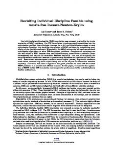
II. Background: EGO using Probability of Improvement A brief description of Efficient Global Optimization (EGO) algorithm developed by Jones et al. 18 is provided, followed by a description for Probability of targeted Improvement (PI) and the optimization of PI. A. Efficient Global Optimization (EGO) Firstly an initial set of data points is fitted with a Kriging model as a realization of a Gaussian Process with a mean of ŷ(x) and a standard deviation of s(x). In this work we use Ordinary Kriging (using DACE toolbox1). Then each cycle consists of selecting additional points based on maximizing EI or PI and refitting the surrogate. Maximizing EI or PI is used here as the selection criteria for new sampling points. Figure 1 illustrates the EGO algorithm using a one dimensional function for EGO-PI. Figure 1(a) shows the data, the kriging fit and its uncertainty, and a target yTarget. Based on the uncertainty model the probability of improving the present best solution (PBS) beyond the target is calculated as explained in subsection B below and shown in Figure 1(b). After adding a new point (near x=0.6 where PI is maximal) to the existing data set, the Kriging model is updated and the process continues until a stopping criterion is met. A similar process is used for EGO-EI and the formulation for EI is explained in Section C. 20 y(x) y Target
15
data y KRG(x)
y
10
PBS
5 0 -5 -10
0
0.1
0.2
0.3
0.4
0.5 x
0.6
0.7
0.8
0.9
1
(a) 0.35 Next point added
0.3 0.25
PI
0.2 0.15 0.1 0.05 0
0
0.1
0.2
0.3
0.4
0.5 x
0.6
0.7
0.8
0.9
1
(b) Figure 1. One cycle of EGO using the probability of improvement (PI) for a one dimensional test function [y(x) = (6x2)2sin(12x-4)] with initial data set as x = [0 0.5 0.68 1]T. The uncertainty (amplified amplitude of 2*s(x)) associated with the kriging is plotted in orange. The target, yTarget is set below the present best solution (PBS).
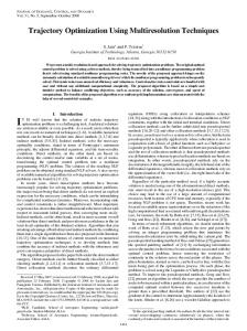
B. Probability of targeted Improvement (PI) The probability of improving the objective beyond a target yTarget at a point x is given by Equation (1)19. This probability is the shaded area in Figure 2(b) which shows the normal distribution of the kriging fit uncertainty at x equal to 0.2.
yT arg et
P I (x )
yˆ(x ) (1)
s(x )
where, Φ (.) is the cumulative density function of a normal distribution, ŷ(x) is the kriging prediction, s(x) is the prediction standard deviation (square root of the kriging prediction variance). 20
y(x) y
15
Target
data yKRG(x)
10
y
PBS 5 0 -5
-10
0
0.1
0.2
0.3
0.4
0.5 x
0.6
0.7
0.8
0.9
1
(a) Kriging estimate at x = 0.2 0.035
Probability distribution of Kriging estimate Kriging estimate y^ (x) Target
0.03
PDF
0.025 0.02 0.015
Shaded Region: PI
0.01 0.005 0 -40
-30
-20
-10
0
10
20
30
40
50
60
(b) Figure 2. Example for illustrating Probability of targeted Improvement of PBS beyond the target at x = 0.2 for a one dimensional test function (same as in Figure 1) with (a) Kriging fit with uncertainty estimates, and (b) Normal distribution of Kriging fit with uncertainty at x=0.2 showing the Probability of targeted Improvement.
C. Expected Improvement (EI) The popular way of selecting points is to maximize the expected improvement (EI)19 upon the Present Best Solution (PBS), yPBS. In this case yPBS is given by the lowest mean of the collected data. EI is given by,
y yˆ ( x) yPBS yˆ ( x) EI ( x) ( yPBS yˆ ( x)) PBS s ( x) s ( x) s ( x) where, ϕ(.) is the probability density function of a normal distribution.
III. Optimization when simulation cost is comparable to the objective function In this work, two cases are checked when cost of function evaluation is comparable to the objective function. The first case deals with limited budget and the second case incorporates the cost as a significant part of the objective function.
(2)
A. Fixed budget Fixed budget involves setting the total number of available function evaluations to a fixed number. The EGO algorithm balances exploration and exploitation, with exploration cycles focusing on sparsely explored regions and exploitation cycles refining the search in known good regions. We assume that as we get close to exhausting our budget, exploration should cease, and it may be better to do pure exploitation, that is, evaluate the objective function at the minimum of the surrogate. That is, for a given budget, we investigate if it is best to use the adaptive sampling strategy of EGO-EI, using both the surrogate prediction and uncertainty, for the entire budget or switch to a pure exploitation of the surrogate prediction using DE23 optimizer. The DE optimization is implemented with 4 starts in this work. B. Cost as a significant part of the objective function The formulation of the optimization problem with cost as a part of the objective function (J) is given by,
min x, N
J f ( x) N
(3)
where, f(x) is the actual objective function, α is the cost associated with each simulation, and N is the number of simulations. αN represents the cost of optimization. The optimization is carried out by using EGO with PI as the selection criterion. Since an improvement in J requires at least an improvement of α in f in the next cycle, the target value for PI is set as α below the Present Best Solution (JPBS) as given by, (4)
J Target J PBS
A stopping criterion could be devised based on the cost of simulation. In this case, a low probability of achieving the target, JTarget, is used to decide termination of optimization algorithm as given by Equation (5) for EGO cycle k.
PI k PI Stop
(5)
This means that if the probability of achieving an improvement of α in the next cycle is below PIStop, then the optimization is stopped. Different values of α and PIStop are explored in this work. In order to compare the efficiency of the stopping criterion for different values of cost (α) and PIStop, the distance of the value of JPBS at the terminating EGO cycle from the actual minimum of JPBS is checked considering if the algorithm was run for a longer time. This 𝑖 distance for DOE i is given by 𝑑𝑚𝑖𝑛(𝐽 . 𝑃𝐵𝑆 ) i * d min( J PBS ) J PBS ( xT , kT ) min( J PBS )
i
(6)
𝑖 where, 𝑥 𝑇∗ is the location of best solution obtained in the terminating EGO cycle kT. The distance 𝑑𝑚𝑖𝑛(𝐽 𝑃𝐵𝑆 ) reflects the deficiency or imperfection in the stopping criterion, so the smaller it is, the higher is the efficiency of the stopping criterion.
IV. Results and Discussion We employed the two dimensional modified Branin and Sasena functions to test the case of limited budget (more details on these functions in Appendix A) and the Sasena function for the case of including cost as a part of the objective function. To average out the influence of the design of experiment (DOE), 50 different Latin Hypercube 24 DOEs were created using MATLAB function lhsdesign. A. Results for fixed budget The results are tested for initial DOE sizes of 5 and 8 sample points for both functions. We used EGO-EI in this case and investigated switching after every optimization cycle for different given budgets, nbudget, of 11, 13, 15, 18 and 23 function evaluations. The number of function evaluations is given by the initial DOE size added to the number of optimization cycles. In EGO the maximization of EI is done using DE23 optimizer with 4 starts. The DE optimizer used for pure exploitation of surrogate prediction is also implemented with 4 starts. The modified Branin and Sasena functions along with their local optima are plotted in Figure 3. It can be clearly seen that the different optima for modified Branin function are very competitive especially when the large range of the function is taken
into account. On the other hand, Sasena clearly has one global optima with the other local optima not being competitive in comparison (also has smaller range of the function compared to modified Branin). Sasena
Modified Branin 5
15
250
10
35
X= 4.71 Y= 5 Level= 33.2423
4.5
30
4
X= -3.15 Y= 12.3 Level= -4.9168
X= 2.5 Y= 2.58 Level= -1.4564
x2
x2
3 150
X= 3.78 Y= 3.98 Level= 12.6896
3.5
200
25
20
2.5 15
2 5
100
X= 9.41 Y= 2.46 Level= -3.6601
X= 3.13 Y= 2.28 Level= -4.2885
X= 0.18 Y= 1.97 Level= 2.8663
1.5
10
1 50
5 0.5
0 -5
0
5
0
10
0 0
1
2
3
x
x
(a)
(b)
1
4
5
1
Figure 3. Plots of (a) modified Branin and (b) Sasena functions along with their local optima
The results for the modified Branin function while switching to DE from EGO-EI after certain number of function evaluations for different budgets as a median of 50 DOEs of sizes 5 and 8 can be found in Figure 4 and Figure 5, respectively. Switching in the first optimization cycle (number of function evaluations equal to DOE size) indicates no adaptive sampling was done. The first data in each case (‘No Switch’) refers to the case when only adaptive sampling was used for the entire budget. It can be seen that for low budgets (≤15), the best results can be achieved by just using pure exploitation of surrogate predictions. For larger budget of 23 it can be seen that switching to DE too soon would lead to getting stuck at a local optimum. The adaptive sampling gives very close to the best result which is found if we switch after around 15 function evaluations, indicating that for larger budgets sticking to adaptive sampling is a good strategy. For modified Branin, as discussed before, the local optima are very competitive, which shows the advantage of using adaptive sampling at least for a few optimization cycles if sufficient budget is available in order to escape a local optimum Modified Branin with different budgets for DOE size of 5
Median best optimum for given budget
-2.5
n
= 11
n
= 13
n
= 15
n
= 18
n
= 23
budget budget
-3
budget budget
-3.5
budget
Global Optimum -4
-4.5
-5
No Switch
6
8
10
12
14
16
18
20
22
Function evaluations when switched to DE
Figure 4. Best optimum obtained at the end of the given budget when switching to DE from EGO-EI after certain number of function evaluations as a median of 50 DOEs of initial size 5 for Modified Branin function (‘No Switch’ indicates the case when EGO-EI is used for the entire budget)
Modified Branin with different budgets for DOE size of 8
Median best optimum for given budget
-1.5
n
= 11
n
= 13
n
= 15
n
= 18
n
= 23
budget
-2
budget budget
-2.5
budget
-3
budget
Global Optimum -3.5
-4
-4.5
-5
No Switch 8
10
12
14
16
18
20
22
Function evaluations when switched to DE
Figure 5. Best optimum obtained at the end of the given budget when switching to DE from EGO-EI after certain number of function evaluations as a median of 50 DOEs of initial size 8 for Modified Branin function (‘No Switch’ indicates the case when EGO-EI is used for the entire budget)
The results for the Sasena function while switching to DE from EGO-EI after certain number of function evaluations for different budgets as a median of 50 DOEs of sizes 5 and 8 can be found in Figure 6 and Figure 7, respectively. For sparser DOE of size 5, using adaptive sampling for smaller budgets (


![Cost Optimization Pillar [PDF]](https://m.moam.info/img/260x300/cost-optimization-pillar-pdf_6479b31b098a9e2a3a8b457b.jpg)