Reliability Based Design Optimization Using First, Second ... - AIAA ARC

Reliability Based Design Optimization Using First, Second and Quasi-Second Order Saddlepoint Approximations Dimitrios I. Papadimitriou1, Dionysios N. Panagiotopoulos2 and Zissimos P. Mourelatos3 Oakland University, Mechanical Engineering Department, Rochester, MI, 48309

A new reliability-based design optimization (RBDO) approach is proposed based on saddlepoint approximation. An extension of the existing first-order saddlepoint approximation is proposed using a second-order Taylor expansion of the limit state function. This expansion utilizes curvature information from the Hessian matrix, resulting in a more accurate prediction of the probability of failure. The expansion is performed at the mean values of the random parameters increasing the efficiency of the so-called mean-value second-order saddlepoint approximation (MVSOSA) method. To improve computational efficiency, the implementation of MVSOSA in RBDO, estimates the exact Hessian matrix only at selected optimization cycles, based on how much the design changes from the previous iteration. The methodology is first demonstrated using two mathematical examples, and then applied to the reliability-based design optimization of two beams, minimizing their weight under probabilistic constraints. It is demonstrated that the proposed RBDOMVSOSA method is more efficient than other methods in the literature, maintaining highaccuracy in estimating the probability of failure.

I. Introduction

Q

UALITY improvement of products is based on how parts are designed to maintain adequate reliability. A lot of research has been conducted on estimating reliability effectively and accurately. Monte Carlo simulation (MCS) is an accurate method but very expensive. First and second order reliability methods (FORM and SORM)1,2 use linear and quadratic approximation of the limit state functions respectively. FORM is accurate and efficient with linear limit states whereas SORM may be used when the nonlinearity of the limit states is high. These two methods are the most common in the literature. If variability and/or uncertainty is present, RBDO provides safer and less expensive designs than deterministic design optimization because it efficiently accounts for variability using probabilistic theory. As a result, RBDO is being increasingly accepted as an effective design tool for aerospace, automotive and civil engineering structures. An overview of RBDO is readily available in the literature (e.g. Frangopol et al.3) with applications in the design of aerospace, civil and mechanical systems, among others. A designer faces many challenges when applying RBDO to practical problems. The high computational cost and the accuracy in estimation of failure probability are two principal challenges that this paper tries to address. Calculating the probability of failure for a design requires repeated analyses for different realizations of the random variables, which may be computationally expensive, especially when finite element analysis is required4-6. Furthermore, the computational cost is compounded when calculating the probability of failure of different designs during the search for the optimum reliability-based design. To reduce the computational cost of conventional double-loop (DLP), sequential optimization and reliability assessment (SORA), and the single loop approach (SLA) approaches have been proposed5-15. The DLP approach uses one optimization loop to calculate the optimal values of the design variables (outer loop), and an inner loop to calculate the most probable point (MPP) of each probabilistic constraint. SORA decouples the RBDO process into a sequence of cycles consisting of deterministic design optimization followed by a reliability assessment of the optimum7. The constraints in the deterministic optimization dictate that the design does not fail at a checking point, which is an approximation of the MPP. The SORA7 method uses the reliability information from the previous cycle 1

Research Associate, Department of Mechanical Engineering, [email protected]. PhD Candidate, Department of Mechanical Engineering, [email protected], Student Member AIAA. 3 Professor, Department of Mechanical Engineering, [email protected], Member AIAA. 1 American Institute of Aeronautics and Astronautics 2

to shift the violated deterministic constraints in the feasible domain8. Another decoupled approach has been proposed9, restricted to deterministic design variables in the design optimization loop. An adaptive sequential linear programming (SLP) algorithm has also been reported10 which employs a filter-based SLP algorithm in order to balance accuracy, efficiency and convergence behavior. Another class of RBDO methods converts the problem into a single-loop, deterministic optimization by integrating the two optimization loops into one11-17. The Saddlepoint Approximation (SA) approach18-19 has recently been applied to reliability analysis20-23. A Firstorder Saddlepoint Approximation (FOSA) method20 linearizes the limit state function at the Most Likelihood Point (MLP) in the original space. In order to avoid the optimization algorithm required to compute the probability of failure, an MVFOSA approach was proposed21, linearizing the limit state at the mean values of the input random variables instead of the MLP. A SA method based on sampling and the extension of SA to system reliability have also been proposed22,23. An improved third-moment saddlepoint approximation has also been reported24. Also, an extension to reliability analysis using a second-order SA has been proposed25, whereas the SA has been applied to reliability-based topology optimization26. This paper proposes the implementation of a new Mean-Value, Second-order Saddlepoint Approximation (MVSOSA) into an RBDO framework. The proposed RBDO-MVSOSA methodology uses a second-order Taylor expansion of the limit state function at the mean point of the input random variables. The paper compares its efficiency and accuracy with the first-order RBDO-MVFOSA approach, as well as with the conventional RBDOFORM method and other existing RBDO approaches. During the application of RBDO, the exact Hessian matrix, whose computation comprises the main part of CPU cost of the MVSOSA method in large scale applications, is computed only at selected optimization cycles, when the design changes are large. For the remaining optimization cycles, the Hessian matrix is approximated with that of the previous optimization cycle. The paper is organized as follows. Section II provides a brief introduction to RBDO, MVFOSA and MVSOSA methods. It also describes how to obtain sensitivity information needed in RBDO. Section III provides details on the proposed RBDO approach, and all its variants, using MVSOSA. The latter evaluates the probabilistic constraints. Section IV demonstrates the accuracy and efficiency of the proposed method using various examples. Finally, a summary and conclusions are presented in Section V.

II. Overview of Reliability-Based Design Optimization (RBDO) A. General Formulation An RBDO problem is typically formulated as

min f d, μ X , μ P 

d, μ



Χ



s.t R i  P Gi d, X, P   0  Ri , for i  1,...,n L

U

t

L

(1)

U

d  d  d , μX  μX  μX

where d  R is the vector of the deterministic design variables, X  R k

m

is the vector of random design variables,

q

and P  R is the vector of random parameters. A bold letter indicates a vector, an uppercase letter indicates a random variable or a random parameter, and a lowercase letter indicates a realization of a random variable or t

random parameter. R i  1  p f denotes the actual reliability level of the ith constraint and Ri denotes the i

corresponding minimum allowable reliability. Gi d, X, P  defines the limit state function of the ith constraint. The system fails if Gi d, X, P  becomes negative and survives if it is non-negative. The optimization problem of Eq.(1) is usually solved using a double-loop (DLP) RBDO approach that employs two nested optimization loops, the design optimization loop (outer) and the reliability assessment loop (inner). The latter is needed for the evaluation of each probabilistic constraint. If the probability of failure is estimated using FORM, at each optimization cycle the design optimization loop calls for a constraint evaluation, where a reliability 2 American Institute of Aeronautics and Astronautics

assessment loop is executed that searches for the MPP in the standard normal space. If the random variables are nonnormal, a non-linear transformation maps the original space to the standard normal space. The remainder of this section highlights the first and second-order saddlepoint approximation methods. The proposed RBDO methodologies, based on second-order saddlepoint approximations are presented in section III. They can be considered as single-loop methods, since the computation of the probability of failure does not require an inner optimization loop and, thus, the efficiency is expected to increase. Also, because there is no need for transformation to the standard normal space, the proposed method is expected to compute the probability of failure accurately.

B. Mean-Value First-Order Saddlepoint Approximation (MVFOSA) The First-Order Saddlepoint Approximation (FOSA)20 linearizes the limit state function at the Most Likelihood Point (MLP) in the original space, in contrast to the First-Order Reliability Methods (FORM) which linearize the limit state in the standard normal space. In doing so, FOSA does not use a transformation to the standard normal space which would increase the nonlinearity of the limit state function. The Mean-Value First-Order Saddlepoint Approximation (MVFOSA)21 is a more efficient, although potentially less accurate, alternative to FOSA. Instead of linearizing the limit state at the MLP, it linearizes it at the mean point of the input random variables avoiding therefore the solution of an optimization problem to locate the MLP. Note that MVFOSA is more accurate than MVFOSM (Mean-Value, First-Order, Second Moment) with the same computational cost, and in certain cases it is more accurate than FORM because it does not use a transformation to standard normal space. MVFOSA is summarized below for completeness. In MVFOSA, the linearization of the limit state function g at the mean values of the random variables is very convenient because it allows the computation of the Moment Generating Function (MGF) of the limit state function directly from the MGFs of the input random variables. However, the accuracy of MVFOSA may decrease for problems with large uncertainties, i.e. large coefficient of variation (COV) for the input random variables, as the examples of Section IV indicate.

1. Estimation of probability of failure using RBDO-MVFOSA The MGF of a random variable X is given by

M X t  







etx f X x dx

(2)

where f X x  is the Probability Density Function (PDF) of X . If the MGF is known, all statistical moments of can be calculated. The Cumulant Generating Function (CGF) is the logarithm of the MGF K X t   lnM X t  .

X

(3)

If Y  g X , i.e. the limit state g is a function of the random vector X, MVFOSA linearizes g at the mean values





μ   X 1 , ,  X n of X  X1, ,

X n  as

Y  g μ  

g  X X n

i 1

where

g X i

i

 Xi



(4)

i μ

are the derivatives of g evaluated at their mean values. Eq. (4) yields μ

 Y   g μ    

n

 i 1

 g Xi    X i μ 

n

 i 1

g X i  a0  X i μ

n

a X i

i 1

3 American Institute of Aeronautics and Astronautics

i

(5)

where a0  g μ  

n

g

 X i 1

i μ

 X i and ai 

g . Thus, the MGF of Y is X i μ

M Y (t )  e

ta0







n  t   a i xi  i 1   e

f X x1,, x n dx

(6)

Eq. (6) is general and applicable to any type of random variables considering also their correlation structure. If the random variables are independent, Eq. (6) yields MY (t )  eta0 M X1 (a1t )  M X n (ant )

(7)

Similarly, the CGF of Y is

KY t   lnM Y (t )  a0t 

n

K i 1

   g     

n

 i 1

g X i

Xi

ait  

  X i t    

 g  KXi  t  X i  i 1    n



(8)

where K X i t  is the CGF of X i . Eq. (8) provides the CGF of the limit state in terms of the CGFs of the random variables. If the CGF of g is known, the probability of failure is approximated as (Lugananni et al.27)  1 1 Pf  PY  y   w   w   w v

(9)

where  and  are the CDF and PDF of the standard normal distribution,

w  sgnts 2ts y  KY ts 1 2

(10a)

v  ts K ts 1 2 .

(10b)

and

t s is the saddlepoint which is computed from the solution of the solution of K t s  and K t s 

K ts   y . (11) in Equations (11) and (10b) respectively, are the first and second-order derivatives of the

CGF with respect to t , evaluated at t s . They are given by

KY t   a0 

n

a K

ait 

(12)

 a  K  a t  .

(13)

i

i 1

Xi

and

K Y t  

n

2

i

i 1

Xi

i


The main advantage of the MVFOSA is its simplicity and low cost. The latter depends however, on the availability of the gradient of g with respect to X. If the limit state is a “black-box” function, the gradient is computed using finite differences with a cost proportional to the number of random variables. Thus, the cost to estimate the probability of failure Pf using MVFOSA if finite differences are used is almost equal to the cost of evaluating the limit state function as many times as the number of random variables. Otherwise, an adjoint method 30 can be used to compute the gradient efficiently. The cost of the adjoint approach (either in its discrete or continuous form), is equivalent to the cost of solving the state equations and is independent of the number of random variables. Thus, if an adjoint approach is used, the cost to estimate the probability of failure Pf is only equal to twice the cost of evaluating the limit state function, regardless of the number of random variables. On the other hand, the accuracy of MVFOSA may reduce if the standard deviations of X i , i  1,, n are large and the limit state function is strongly non-linear. This paper alleviates this drawback by implementing a secondorder Taylor expansion of g.

2. Sensitivity Analysis for RBDO-MVFOSA In RBDO using MVFOSA, the first-order sensitivity derivatives of Pf with respect to the design variables are needed. In general, the design variables comprise the deterministic variables and the mean values of the random variables. Differentiation of Eq. (9) provides the gradient of Pf with respect to the design variables  i as

Pf i



 1 w 1 v  w  w  1 1     2      w  2  i i  w v   w i v i 

(14)

where

 t w y KY ts    sgnts ts y  KY ts 1 2  s y  ts   i i i   i

(15)

v t 1 K ts   s K ts 1 2  ts K ts 1 2 . i i 2 i

(16)

and

The sensitivities

t s of the saddlepoint are computed by solving the equations  i

K ts  0 i

(17)

The derivatives of K ts  , K ts  and K t s  with respect to the design variables are

K ts  a0 t  ts  a0 s   j  j  j

  K X ait   i j i 1   ai  K X i ai t    n  K t s  a0  j      ai   j i i 1  t  ai  t s  ai s  K X i ait    j    j     n

 ai

 

ts  ai

ts  j




(18)

(19)

and K ts    j



n

ai

 2a  i 1

i



j

 a t K X i ait   ai2  i t s  ai s   j  j 

   K X ait  i   

(20)

Eq. (17) is linear and can be solved directly to obtain

t s   j

a0  i

 ai

n

   i 1

K X i ait   ai

j

 n

i 1

ai2 K X i

 ai t s K X i ait   j 

ait 

Note that since ai depends on the gradient of g with respect to the random variables, the computation of

(21)

ai  j

requires a second-order sensitivity analysis. This can be done using efficient second-order direct differentiation or adjoint approaches, depending on the specific problem. For instance, if the number of random variables is much less than the number of design variables, direct-differentiation is preferable for the random variables, and the adjoint approach is preferable for the design variables. Thus, the computational cost depends only on the number of random variables and is independent of the number of design variables.

C. Mean-Value Second-Order Saddlepoint Approximation (MVSOSA) In this section, we present a Mean-Value, Second-Order Saddlepoint Approximation (MVSOSA) method, to be used in an RBDO-framework. MVSOSA improves the accuracy of MVFOSA by approximating the limit state with a second-order Taylor expansion, including the Hessian matrix of the limit state function with respect to the random variables.

1. General Formulation for MVSOSA A second-order Taylor expansion of g at the mean values of the random variables yields

Y  g μ  

g  X X n

i 1

1  2

i



 Xi 

i μ

n

2g X i X j j 1

X i   X X j   X 

n

 i 1

i

.

(22)

j

μ

Eq. (22) requires the Hessian matrix of g with respect to the random variables. The Taylor expansion can be applied at the MLP resulting in a more accurate but less efficient SOSA method. The methodology proposed below is generic and can be applied to SOSA as well. In this paper, we use MVSOSA because of its computational advantage over SOSA. The second-order expansion of g yields   n n n g 1 2g   Y   g μ   Xi  Xi X j   X i μ 2 i 1 j 1 X i X j   i 1 μ     n n n n 2g 1 2g  g   X j X i  Xi X j  X  X i X j 2 i 1 j 1 X i X j  i μ i 1  j  1 μ μ  












(23)

and can be expressed as the following quadratic function Y  Q(X)  XT AX  bT X  c

(24)

where

Aij 

1 2g g , bi  2 X i X j X i μ

c  g μ  

n

 i 1

g 1 X  X i μ i 2

2g

n

 μ n

 X X j 1

i

X j , j μ

(25)

n

2g Xi X j X i X j j 1

 i 1

μ

The MGF of Y is now expressed as M Y (t ) 







etQ( x) f X xdx .

(26)

In contrast to MVFOSA where the MGF can be expressed in terms of the MGFs of the random variables (Eq. (6)), in MVSOSA the integration of Eq. (26) cannot be performed analytically for non-Gaussian distributions in a straightforward manner.

2. MVSOSA for Gaussian random variables If X ~ N (μ, ) is a normal vector with mean μ and covariance  , the MGF of the quadratic function Q(x) is given analytically28 in terms of t, as 

M Y (t )   etQ ( x ) f X xdx  B

1 2





exp t μ  Aμ  b μ  c   t 2 2dT B 1d



(27)

where B  I  2t1 21 2

(28)

d  1 2b  21 2 Aμ .

(29)

and

Thus, the CGF of Y (logarithm of MGF) is



  

1 KY (t )   log B  t μ Aμ  bμ  c  t 2 2 dT B 1d . 2

(30)

The above analytical expression of CGF allows for the computation of its first and second-order derivatives, required for saddlepoint approximation, as 1 KY (t )   trace B 1 B  μ  Aμ  b μ  c 2 (31) T 1 2 T 1 1   td B d  t 2 d B B B d and 1 KY (t )  trace B 1BB 1B  dT B 1d . (32) 2  2tdT B 1BB 1d  t 2dT B 1BB 1BB 1d

  







Note that prime (  ) indicates differentiation with respect to t. To derive Equations (31) and (32), the following expressions for the derivatives of inverse matrices and determinants are used


B   B 1



 

  BB 1 , B1  2B1BB1BB1  B1BB1 , B  B trace( B 1B) ,

1



B  B trace( B 1B)  B trace( B 1BB 1B  B 1B) , B  21 2 1 2 and B  0 .

(33)

3. Sensitivity analysis for RBDO-MVSOSA The computation of Pf requires up to second-order sensitivity derivatives with respect to the random variables. Furthermore, similarly to MVFOSA, the derivatives of Pf with respect to the design variables are needed in RBDO if a gradient optimizer is used. Thus, mixed third-order sensitivity derivatives are needed, including twice differentiation with respect to the random variables and once with respect to the design variables. The derivatives of KY ts  , KY ts  and KY ts  with respect to the design variables  i at the saddlepoint t s are expressed as  K Y (t s ) t 1 B  K Y (t )  trace B 1  i  i 2  i 

 

 A bT c  t μ  μ μ      i i i 

T 1    t2 2  d B d   i 



  B 1 B K Y (t s ) t 1  K Y (t )  trace    i  i 2 i 





1

  

b c d B d μ t  t2  i  i  i T

  μ  



1













(34)

A μ  i



T

(35)

   

d B d  d B BB 1d  dT B 1BB 1BB 1d   2t  t2 i i i T

1



 d B BB 1d 2  i T

  B 1BB 1B KY (ts ) t 1  KY(t )  trace  i i 2 i  1

   



(36)

The third derivative of KY t  with respect to t in Eq. (36) is given by





KY(t )  trace B 1BB 1BB 1B  3dT B 1BB 1d  6td B BB BB d  3t d B BB 1BB 1BB 1d T

1

1

1

2 T

1

.

(37)

Using finite differences to compute these derivatives may be computationally demanding and accuracy issues may arise due to sensitivity with the step size. If the limit state is not a “black-box” function, a high-order adjoint method can efficiently compute high-order sensitivities. The efficient combination of direct-differentiation and adjoint methods to compute third order sensitivities has been presented for topology optimization26,29 and for CFD applications30.

III. Proposed RBDO-MVSOSA algorithm In large scale problems, the cost to compute the probability of failure using MVSOSA comes mainly from computing the gradient vector and especially the Hessian matrix of the limit state function with respect to the random variables. If finite differences are used, the computational cost scales with the square of the number of random variables, increasing the total cost prohibitively. Alternatively, second-order adjoint methodologies may be used, combining the adjoint method with direct-differentiation of the state equations31, to reduce the overall computational cost which can scale linearly with the number of random variables. 8 American Institute of Aeronautics and Astronautics

A. Constant Hessian RBDO-MVSOSA (CH-RBDO-MVSOSA) For problems with many random variables, even the linear dependence of the cost of Hessian matrix computation to the number of random variables makes the MVSOSA approach quite expensive, compared to the first-order reliability methods and MVFOSA. To make matters worse, in RBDO problems, the Hessian matrix must be computed at each optimization cycle. In order to alleviate this problem, we propose computing the exact Hessian only at the first optimization cycle of the RBDO, and keep it constant for subsequent cycles. This methodology, called Constant RBDO-MVSOSA or CH-RBDO-MVSOSA, is expected to be very accurate if the Hessian matrix does not change too much. For many problems, this is true if the RBDO approach starts with the deterministic optimum, which is expected to be relatively close to the RBDO optimum.

B. Constant Hessian - Constant Gradient RBDO-MVSOSA (CH-CG-RBDO-MVSOSA) To increase the efficiency even more, a Constant Hessian-Constant Gradient RBDO-MVSOSA or CH-CGRBDO-MVSOSA is also proposed. It uses the gradient and exact Hessian only at the first optimization cycle of the RBDO procedure, keeping both the gradient and the Hessian constant for subsequent cycles. This method is less accurate than CH-RBDO-MVSOSA, because the latter updates the gradient at every optimization cycle. However, it can be almost as efficient as the deterministic optimization method. As the mathematical examples of Section IV show, the accuracy of CH-CG-RBDO-MVSOSA is very similar to the original RBDO-MVSOSA.

C. Updated Hessian RBDO-MVSOSA (UH-RBDO-MVSOSA) There may be problems however, where the deterministic optimum may be quite far from the reliable optimum, resulting in large changes in the Hessian matrix. For such cases, a modified algorithm is proposed using the exact Hessian matrix only at selected optimization cycles. The selection of these cycles depends on an estimate of how much the design is changed. For that we use the difference of the gradient vector norms between adjacent cycles. The Hessian matrix H is computed if and only if the relative difference of the norm of the gradient vector of the limit state function(s) f for the i  1 constraint from the corresponding norm f i is greater or equal to a user defined percentage difference  % , i.e. f

i

 f f

i 1

  %, i  1, , n

(38)

i

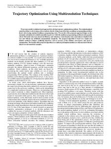
where n is the number of constraints. The percentage  % controls the balance between accuracy and efficiency. The higher the  % is, the higher the expected efficiency and lower the expected accuracy of the Updated Hessian RBDO-MVSOSA (UH-RBDO-MVSOSA) becomes. Thus, if  % is large, the algorithm in Fig. 1 will calculate the Hessian H fewer times, and is expected to converge faster. However, it may be less accurate. In contrast, if  % is low the algorithm will calculate H more often and the accuracy will increase at the expense of a higher computational cost. Fig. (1) shows a flowchart of the RBDO-MVSOSA methodologies with constant or updated Hessian matrix.


Initialize d, μ X

Compute

f

i

Gi Gi , X P

 f f

i 1

 %

i

True

False

H i 1  H old

Calculate H i 1

Compute:

f , Pf

Update: d, μ X

Compute

f f Pf Pf , , , , μ X d μ X d

False Convergence?

True Stop Figure 1. Flowchart of proposed RBDO-MVSOSA methods 10 American Institute of Aeronautics and Astronautics

D. Computation of First and Second-Order Derivatives - Methods and Efficiency The estimation of the probability of failure using MVFOSA requires the computation of the limit state function and its gradient with respect to the random variables computed at their mean values. The gradient of the limit state function may be computed either with finite differences or using the adjoint approach. In the former case, which is preferred for black-box problems, the gradient computation requires as many function evaluations as the number of variables. The expression of first-order central finite differences is as follows g X i



g ( X 1 ,..., X i   ,..., X N )  g ( X1 ,..., X i   ,..., X N )

(39)

2

If the adjoint approach31 is employed, the cost to compute the gradient with respect to random variables is equal to the cost of one function evaluation irrespective of the number of random variables. Table 1 summarizes the cost of finite differences and adjoint approach in terms of function evaluations. It should be noted that the number of constraint evaluations for the applications of Section IV refers to finite differences, for consistency in comparisons with other RBDO methods. Table 1. Cost of gradient, Hessian and failure probability computation Function Evals. (Central Finite Differences)

Function Evals. (Adjoint)

Gradient

2N

1

Hessian

2N(N-1)

N

Total Cost, MVFOSA (Function and Gradient)

2N+1

2

Total Cost, MVSOSA (Function, Gradient and Hessian)

2N2+1

N+2

N is the number of random parameters and random variables To compute the probability of failure using MVSOSA, the estimation of the Hessian matrix of the second-order derivatives of the limit-state functions with respect to the random variables is also required. If second-order finite differences are used to estimate the Hessian matrix, 2N(N-1) additional constraint function evaluations are required. This number is based on the following second-order central finite differences for the Hessian of the limit state function 2

 g 2 X i



2

 g X i X j

g ( X 1 ,..., X i   ,..., X N )  2 g ( X 1 ,..., X i ,.., X N )  g ( X 1 ,..., X i   ,..., X N )





2

g ( X 1 ,..., X i   ,..., X j   ,..., X N )  g ( X 1 ,..., X i   ,..., X j   ,..., X N ) 4

2

g ( X 1 ,..., X i   ,..., X j   ,..., X N )  g ( X 1 ,..., X i   ,..., X j   ..., X N ) 4

2


, for i  j



(40)

Alternatively, especially for large scale problems, the Hessian matrix may be computed by high-order adjoint approaches34. In that case, its computation requires N additional constraint function evaluations. The cost for the Hessian matrix using finite differences and the adjoint method is summarized in Table 1.

IV. Applications A. Mathematical example 1 This section presents a mathematical example to demonstrate the accuracy and efficiency of the proposed RBDO-MVSOSA methods compared to existing RBDO methods such as RIA, PMA, SLSV and SORA. The results for the existing RBDO methods are obtained from Cho and Lee32 and Lee and Lee33. The objective function and the three probabilistic constraints, expressed in terms of the two statistically independent and normally distributed





random design variables X i ~ N  X i ,0.3 , define the RBDO problem as follows 2

min f   X1   X 2

 X1 ,  X 2





such that P Gi X   0  1  p fi for where

G1 X   1 

t

i  1,..,3

2

X1 X 2 20

2 2   X 1  X 2  5 X 1  X 2  12  G X   1   2

G3 X   1 

0.0   Xi  10.0 ,

X

t p fi

30 80

2 1

 8X 2  5

(41)

120



 0.0013 , for i  1,..,3

The deterministic optimization requires 4 cycles to converge, including the computation of the objective and constraint functions 15 times each (Table 1). It starts from an initial point  0X  [2.1, 1.5]T . The deterministic i

optimum  X  [3.10, 2.09] is used as a starting point for all RBDO methodologies. The convergence criterion is 0

T

i

equal to 10−3 . The convergence histories of the objective function for the RBDO problem are shown in Fig. 2a. The optimization converges in 8 cycles. Fig. 2b shows the convergence histories of the two active reliability constraints. The constraints become active after the fourth cycle and remain active until convergence. In Table 1, the optimal values of the design variables and the corresponding objective function are reported for each method. The table also shows the number of objective and constraint function evaluations, required for convergence. Table 2 compares the probabilities of failure at the optimal point of the RBDO problem.


7.4

Objective Value

6.9 6.4 5.9

RBDO-MVFOSA

5.4

RBDO-MVSOSA

4.9

CH-RBDO-MVSOSA UH-RBDO-MVSOSA (5%)

4.4

CG-RBDO-MVFOSA

3.9

CH-CG-RBDO-MVSOSA 3.4 0

2

4

6

Iteration Number

8

10

Figure 2a. Convergence history of objective function

RBDO-MVFOSA

0.5013

RBDO-MVSOSA 0.4013


0.3013

CG-RBDO-MVFOSA

0.2013

CH-CG-RBDO-MVSOSA

0.1013

0.0013 0

2

4

6

Iteration Number

8


10

RBDO-MVFOSA

0.5013

RBDO-MVSOSA 0.4013


0.3013

𝑝𝑓2

CG-RBDO-MVFOSA CH-CG-RBDO-MVSOSA

0.2013

0.1013

0.0013 0

2

4

6

Iteration Number

8

10

Figure 2b. Convergence history for the two active probabilistic constraints The 8 optimization cycles required by RBDO-MVFOSA include 27 evaluations of the objective function and 27 evaluations of each of the three probabilities of failure. According to Table 2, in the case of RBDO-MVFOSA, the 27 evaluations of the probabilities of failure require 27*(1+2*2) = 135 computations of the limit state functions. The computational cost of the RBDO-MVFOSA method is lower than that of the other RBDO methods. This cost is further reduced if the Constant Gradient RBDO-MVFOSA (CG-RBDO-MVFOSA) method is used, which calculates the G i once at the first iteration and it keeps it constant afterwards. The reduction of the computational cost between RBDO-MVFOSA and CG-RBDO-MVFOSA is 96.3%, with a slight decrease in accuracy of the computed probability of failure (Table 2). However, the accuracy of both RBDO-MVFOSA and CG-RBDOMVFOSA methods is much lower than other existing methods (Table 3). Monte Carlo Simulation (MCS) using 107 simulations is used to validate the computed probability of failure at the optimum. MCS estimates the probabilities of failure at the RBDO-MVFOSA optimum as (7.3e-5, 3.961e-4) instead of (0.0013, 0.0013), and the relative errors are equal to 94.4% and 69.5%. Table 2. Summary of optimization results for example 1 RBDO Method

Obj.

Deterministic RIA PMA SLSV SORA MVFOSA CG-MVFOSA

5.1765 6.7260 6.7280 6.7310 6.7260 7.0863 7.0845

Design Variable (3.1139,2.0626) (3.4390,3.2870) (3.4390,3.2890) (3.4340,3.2970) (3.4390,3.2870) (3.6366,3.4496) (3.6355,3.4489)

H Evals.

Number of Function Evals.

-


Obj.

Constr.

15 16 17 12 33 27 27

15 618 450 153 201 135 5

MVSOSA 6.7196 (3.4444,3.2751) 27 243 27 CH-MVSOSA 6.8000 (3.5030,3.2969) 27 139 1 CH-CG-MVSOSA 6.9000 (3.5604,3.3458) 1 24 14 UH-MVSOSA (5%) 6.7199 (3.4448,3.2752) 27 155 5 * CH stands for constant Hessian, CH-CG for constant Hessian and constant gradient, and UH for updated Hessian Table 3. Comparison of probability of failure at the optimum for example 1

RBDO Method

pf

pf

1

pf

pf

2

2 Rel. error Rel. error with MCS with MCS 0.0014697 0.001133 RIA 13.05% 12.85% 0.0014796 0.001103 PMA 13.82% 15.15% 0.0014806 0.000987 SLSV 13.89% 24.08% 0.0014700 0.001134 SORA 13.08% 12.77% 7.3e-05 3.961e-04 MVFOSA 94.38% 69.50% CG-MVFOSA 7.73e-05 94.05% 4.034e-04 68.97% 0.0014562 0.001302 MVSOSA 12.02% 0.19% 7.2e-04 0.001287 CH-MVSOSA 44.62% 0.98% CH-CG-MVSOSA 3.129e-04 75.93% 9.712e-04 25.29% 0.001290 UH-MVSOSA (5%) 0.0014641 12.62% 0.79% * CH stands for constant Hessian, CH-CG for constant Hessian and constant gradient, and UH for updated Hessian

1

Using the same convergence criterion, MVSOSA requires 8 optimization cycles to converge, and calls the objective and constraint functions 27 times in total. However, each constraint function evaluation also requires the Hessian matrix consisting of the second-order derivatives of the limit-state functions with respect to the random variables. According to Table 1, the estimation of the probability of failure requires in total 2N2+1 limit state function evaluations. In our case, with two random parameters, the 27 computations of the probabilities of failure correspond to 27*(2*22+1) = 27*9 = 243 limit state function evaluations. The efficiency of RBDO-MVSOSA is worse than that of RBDO-MVFOSA but comparable to other existing methods. However, as the last two columns of Table 3 show, the accuracy of MVSOSA is better than that of MVFOSA and other existing algorithms. To increase the efficiency of RBDO-MVSOSA, the CH-RBDO-MVSOSA and UH-RBDO-MVSOSA approaches (Section III) were employed. This time, the Hessian matrix is computed only at selected optimization cycles, reducing the total number of limit state function evaluations. For CH-RBDO-MVSOSA, the Hessian matrix requires (2*2(2-1)) = 4 evaluations and is computed only at the first iteration resulting in 1*9+26*5 = 139 limit state function evaluations (the gradient, computed at all cycles, requires 2*2 = 4 evaluations). Its efficiency is comparable to RBDO-MVFOSA. However, compared to RBDO-MVSOSA, the accuracy is lower (Table 3). The computational cost is decreased even more if both the gradient and Hessian matrix are calculated only at the first iteration and then are kept constant (CH-CG-RBDO-MVSOSA). This method is less accurate than CH-RBDO-MVSOSA, but it is by far the more efficient requiring only 14 constraint evaluations. On the other hand, the RBDO using UH-MVSOSA is more efficient compared to RBDO-MVSOSA with comparable accuracy. The total number of limit state function evaluations is equal to 5*9+22*5 = 155 the exact Hessian is recomputed when the gradient difference between successive iterations is greater or equal to 5%, (5 times for this example). Based on the results from Tables 2 and 3, we conclude that the UH-RBDO-MVSOSA provides the best trade-off between accuracy and efficiency among all tested methods.


B. Mathematical example 2 The proposed RBDO methodology of Section III is herein validated using another mathematical example. Both the objective function and the constraints are quadratic and the random variables X i , i  1,..,10 are statistically





independent and normally distributed as X i ~ N  X i ,0.022 , i  1,...,10 . The RBDO problem is defined as



min f   X2 1   X2 2   X 1  X 2  14  X 1  16  X 2   X 3  10  Xi

  7

2

    3  2  1  5  11  2  10     7   45

 4 X4  5

2

2

2

X5

2 X7

X6

2

X8



2

2

X9

X 10

such that: PG j X  0  1  p tf , j  1,..,8 j where:

G1 X  4 X 1  5 X 2  3 X 7  9 X 8  105 ,

G2 X  10 X1  8 X 2  17 X 7  2 X 8 ,

G3 X  8 X1  2 X 2  5 X 9  2 X 10  12 ,

(42)

G4 X  3 X 1  2  4 X 2  3  2 X 32  7 X 4  120 , 2

2

G5 X  5 X 12  8 X 2   X 3  6  2 X 4  40 , 2

G6 X  0.5 X 1  8  2 X 2  4  3 X 52  X 6  30 , 2

2

G7 X  X 12  2 X 2  2  2 X 1 X 2  14 X 5  6 X 6 , 2

G8 X  3 X 1  6 X 2  12 X 9  8  7 X 10 2

 X i  0 , i  1,..,10 p tf j  0.0013 , j  1,..,8 The initial point for the optimizer is  0X  [2.17, 2.36, 8.77, 5.10, 0.99,1.43,1.32, 9.83, 8.28, 8.38]T . Table 4 i

summarizes the results and compares them with RIA, PMA, SLSV and SORA32,35. Fig. 3 shows the convergence history of the objective function and Fig. 4 shows the convergence history of all active probabilistic constraints. Tables 5 and 6 compare the accuracy of all methods at the obtained optimum. The deterministic optimization requires 3 cycles for convergence including the computation of the objective and constraint functions 37 times each (Table 4). The deterministic optimum is then used as the initial point for all 2

RBDO methods. The convergence criterion was equal to 10 . The RBDO-MVFOSA method requires 10 optimization cycles, satisfying the probabilistic constraint t

p f j  0.0013, j  1,...,8 , as shown in Fig. 3, which includes 130 computations of the objective function and 2,730 computations of each of the 6 probabilities of failure. The CH-RBDO-MVSOSA method requires 10 optimization cycles and 2,910 computations of each of the 6 probabilities of failure. The number of probabilistic constraint evaluations for all RBDO methods is based on central finite differences in computing the gradient and Hessian of the limit state function. Table 4 shows that CG-RBDO-MVFOSA and CH-CG-RBDO-MVSOSA are the most efficient algorithms, whereas RBDO-MVFOSA and CH-RBDO-MVSOSA are more efficient than other RBDO methods except from SORA and CH-CG-RBDO-MVSOSA compared to which, however, they are much more accurate. CH-RBDOMVSOSA is the most accurate method (Tables 5, 6) and RBDO-MVFOSA is the second most accurate compared to existing methods (RIA, PMA, SLSV and SORA). Thus, CH-RBDO-MVSOSA is superior because it has the lowest relative error for all six active probabilistic constraints, and a relatively high efficiency.


Table 4. Summary of optimization results for example 2

RBDO Method

Obj.

Number of Function Evals.

Design Variable

Obj.

Constr.

Deterministic 24.373 (2.158,2.383,8.752,4.903,1.006,1.436,1.303,9.818,8.261,8.401) 37 RIA 27.749 (2.131,2.340,8.711,5.101,0.934,1.467,1.382,9.804,8.147,8.477) 88 PMA 27.749 (2.133,2.336,8.710,5.099,0.931,1.463,1.384,9.806,8.146,8.466) 143 SLSV 27.751 (2.138,2.323,8.705,5.094,0.922,1.449,1.395,9.815,8.154,8.452) 101 SORA 27.750 (2.135,2.330,8.709,5.101,0.930,1.464,1.389,9.810,8.152,8.463) 151 MVFOSA 27.755 (2.135,2.330,8.709,5.102,0.922,1.445,1.389,9.809,8.155,8.474) 130 CG-MVFOSA 27.759 (2.137,2.326,8.708,5.103,0.922,1.447,1.392,9.812,8.159,8.472) 131 CH-MVSOSA 27.760 (2.135,2.331,8.709,5.102,0.922,1.445,1.388,9.809,8.155,8.475) 130 CH-CG27.765 (2.136,2.325,8.708,5.103,0.922,1.447,1.392,9.813,8.158,8.472) 131 MVSOSA * CH stands for constant Hessian, and CH-CG for constant Hessian and constant gradient

37 21,736 29,032 9,784 1,844 2,730 21 2,910

28

Objective Value

27.5 27 26.5

RBDO-MVFOSA

26

RBDO-MVSOSA

25.5

CH-RBDO-MVSOSA

25

CG-RBDO-MVFOSA

24.5 CH-CG-RBDO-MVSOSA 24 0

2

4

6

8

10

Iteration Number Figure 3. Convergence history of objective function Table 5. Comparison of probability of failure at the optimum for example 2

RBDO Method

pf

RIA PMA SLSV

0.0013606 0.0013481 0.0014231

1

pf

2

0.0012284 0.0014611 0.0012896

pf

3

pf

4

pf

5

0.0014322 0.0014709 0.001334 0.0012972 0.0014703 0.0014246 0.0013232 0.0010928 0.0013024 17 American Institute of Aeronautics and Astronautics

pf

7

0.0014198 0.0013493 0.0012592

222

SORA 0.0013368 0.0013477 0.0014416 0.0013704 0.0012984 0.0012861 MVFOSA 0.0012927 0.0012918 0.0013238 0.0013615 0.0014525 0.0013186 CG-MVFOSA 0.0013259 0.0012845 0.0013007 0.0012951 0.0013119 0.0013456 CH-MVSOSA 0.0013024 0.0013081 0.001299 0.0012894 0.0013027 0.0013007 CG-CH-MVSOSA 0.0012989 0.0012844 0.001303 0.0012333 0.0011945 0.0012993 * CH stands for constant Hessian, and CH-CG for constant Hessian and constant gradient Table 6. Accuracy comparison with MC simulation

pf

RBDO Method

pf

1

pf

2

3

pf

4

pf

5

pf

7

Rel. error Rel. error Rel. error Rel. error Rel. error Rel. error with MCS with MCS with MCS with MCS with MCS with MCS RIA 4.66% 5.510% 10.17% 13.15% 02.62% 9.22% PMA 3.70% 12.39% 00.22% 13.10% 09.58% 3.79% SLSV 9.47% 00.80% 01.78% 15.94% 00.18% 3.14% SORA 2.83% 3.607% 10.89% 05.42% 00.12% 1.07% MVFOSA 0.56% 00.63% 01.83% 04.73% 11.73% 1.43% CG-MVFOSA 1.99% 01.19% 00.05% 00.38% 00.92% 3.51% CH-MVSOSA 0.18% 00.62% 00.08% 00.82% 00.21% 0.05% CH-CG-MVSOSA 0.08% 01.20% 00.23% 05.13% 08.12% 0.05% *CH stands for constant Hessian, and CH-CG for constant Hessian and constant gradient

Probability of failure

0.7013

pf1

0.6013

pf2

0.5013

pf3 pf4

0.4013

pf5

0.3013

pf7

0.2013 0.1013 0.0013 0

2

4

6

Iteration Number

8

10

Figure 4. Convergence history of all active probabilistic constraints for CH-RBDO-MVSOSA

C. Cantilevered beam with rectangular cross section In this section, the proposed RBDO-MVSOSA methodologies are applied to the design optimization of a beam under probabilistic constraints. A cantilever beam in vertical and lateral bending8 is considered. The beam is loaded at its tip by vertical and lateral loads Y and X , respectivery. The length 𝐿 is equal to 100 in. The width 𝑤 and 18 American Institute of Aeronautics and Astronautics

thickness 𝑡 of the cross section comprise the set of deterministic design variables. The objective is to minimize the weight of the beam. This is equivalent to minimizing the cross-sectional area f  wt , assuming that the material density and the beam length are constant.

Figure 5. Schematic of beam with rectangular cross section Two nonlinear failure modes are considered. The first failure mode is the yielding at the fixed end of the beam and the other is defined by the tip displacement exceeding the allowable value D0  2.2535 in. The RBDO problem is formulated as

min f  wt w,t





such that: P Gi X   0  1  p fi for t

i  1,2

where:

600   600  2Y  2 X w t   wt G1 w, t , Y , X , R   1

(43)

R





G2 w, t , E , Y , X , L, D0 

2

Y   Z   2   2  Ewt  t  w  3

4L

2

1

D0

1  t  4 , 1  w  4 , p fi  0.00135 for i  1,2 . t

G1 and G2 are the limit state functions corresponding to the two failure modes. The random parameters consist of the yield stress R of the material, the Young’s modulus E and the horizontal and vertical loads, X and Y. The latter are modeled by normal distributions N (40,000,1,000), N (2.9E 7,0.725E 6), N (500,50) and N (1,000,50) ,

respectively. The initial value for all optimization methods was ( w, t )  (2.0,4.0) . The convergence histories for the deterministic and reliability-based design optimization methods are presented 3

in Fig. 6. The relative error for convergence is 10 . Table 7 shows the optimal values of the design variables and the corresponding values of the objective function, as well as the number of objective and constraint function evaluations. For comparison, the probabilities of failure at the optimal points computed by the Monte Carlo method are shown in Table 8.


8.8

Objective Value

8.6 8.4

8.2 8 RBDO-FORM 7.8

RBDO-MVFOSA

7.6

RBDO-MVSOSA UH-RBDO-MVSOSA (10%)

7.4 0

1

2

3

4

5

6

7

8

9

Iteration Number Figure 6a. Convergence history of objective function for beam with rectangular cross section

RBDO-FORM RBDO-MVFOSA RBDO-MVSOSA

0.100135

UH-RBDO-MVSOSA (10%)

0.000135 0

2

4

6

Iteration Number

8


10

𝑝𝑓2

RBDO-FORM

0.700135 RBDO-MVFOSA

0.600135

RBDO-MVSOSA

0.500135

UH-RBDO-MVSOSA (10%)

0.400135 0.300135 0.200135 0.100135 0.000135 0

2

4

6

Iteration Number

8

10

Figure 6b. Convergence history of probabilistic constraints for beam with rectangular cross section Table 7. Efficiency and accuracy comparison for beam with rectangular cross section

RBDO Method Deterministic FORM MVFOSA MVSOSA UH-MVSOSA (10%)

Design Variables w, t 

H Evals.

7.8235 8.6063 8.5747 8.6059

(2.3516,3.3268) (2.3960,3.5919) (2.3843,3.5962) (2.4010,3.5842)

-

8.6091

(2.4052,3.5793)

Obj.

Number of Fun. Evals

24

21 39 30 24

Constraints σ D 21 21 111 698 270 270 792 792

2

24

264

Obj.

264

*UH stands for updated Hessian Table 7 shows that UH-RBDO-MVSOSA is more efficient than RBDO-FORM while RBDO-MVFOSA is quite more efficient than RBDO-MVSOSA. Also, UH-RBDO-MVSOSA is less accurate than RBDO-MVSOSA (Table 8). The trade-off between accuracy and efficiency depends on the frequency in computing the exact Hessian matrix.


Table 8. Accuracy comparison with MC simulation

RBDO Method

pf

pf

1

pf

2 Rel. error with MCS FORM 0.0013678 01.31% 0.0014048 MVFOSA 0.0018727 32.44% 0.0022587 MVSOSA 0.0013779 02.04% 0.0013156 UH-MVSOSA (10%) 0.0013279 01.65% 0.0012126 * UH stands for updated Hessian

1

pf

2

Rel. error with MCS 03.98% 50.36% 02.58% 10.72%

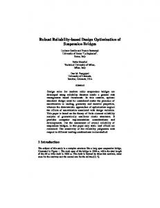
D. Cantilevered I-Beam This section presents an example of a cantilevered beam with an I-shaped cross section loaded by a tip load P (Fig. 7). The beam length is L. The I-shaped cross-section is defined by four parameters, b1 , h1 , b2 , and H .

Figure 7. Schematic of cantilevered I beam The objective is to minimize the volume subject to stress and displacement constraints. The problem has four random design variables which are considered independent normal distributions. The initial point for all RBDO methodologies is H , h1, b2 , b1   7.0, 0.1, 0.1, 9.4 and the convergence error is equal to 10 defined as min

 b1  H ,  b2  h1





0.1   h1

. The RBDO problem is

 

f  2h1 b1   H  2h1 b2  L



such that P Gi X  0 where

2

  1  p tf

G1 X  

P L H

G2 X  

3 PL

i

i  1,..,3

 5,000

2I

 0.065 3EI  1.0 , 0.1  b2  2.0 , 2.0  b1  12.0 , 3.0   H  7.0 t

p fi  0.0027 , i  1,2 22 American Institute of Aeronautics and Astronautics

(44)

I 

1

3  2 1 b1h13  b1h1 H  h1 

2



b2 H  2h1

  

4 12 H , h1, b2 , b1  ~ N H ,0.105, h1 ,0.003 , b2 ,0.0075 , b1 ,0.12 12











Table 9 compares the RBDO-MVFOSA and RBDO-MVSOSA methods if the update frequency of the Hessian matrix is 10%. The number of constraint evaluations for the deterministic optimization is 15 and the corresponding number for RBDO-MVFOSA and UH-RBDO-MVSOSA is 189 and 258, respectively. We note that the UH-RBDOMVSOSA method is more accurate compared to RBDO-MVFOSA while they have a comparable efficiency (number of constraint and objective function evaluations). Table 9. Summary of optimization results for the cantilevered I beam

RBDO Method

H

h1

b2

b1

Objective

Constr. Evals

Objective Evals

pf

Deterministic

7.0

0.1000

0.1

9.48460

92.7692

15

15

0.50370

0.11980

MVFOSA

7.0

0.1162

0.1

9.01370

99.7698

189

21

0.00454

0.00069

UH-MVSOSA (10%)

7.0

0.1207

0.1

8.72830

100.1900

258

26

0.00278

0.00045

pf

1

2

*UH stands for updated Hessian

V. Summary and Conclusions This paper presented a new mean-value second-order saddlepoint approximation (MVSOSA) method for reliability-based design optimization (RBDO). The method extends the mean value first-order saddlepoint approximations (MVFOSA) for reliability analysis to second-order using Hessian matrix information for the probabilistic constraints. The high cost to compute the exact Hessian matrix is alleviated by computing it only at selected optimization cycles. The efficiency of the proposed methodology is comparable to that of MVFOSA and is better than the efficiency of conventional FORM and other existing RBDO methods. In addition to the high efficiency, the probabilities of failure computed by the proposed MVSOSA method with an exact or approximate Hessian matrix are more accurate compared to MVFOSA and FORM. This is demonstrated by two mathematical examples and the design of two cantilevered beams under probabilistic constraints.

References 1

Hasofer, A. M. and Lind, N. C., "Exact and Invariant Second Moment Code Format," Journal Eng. Mech, ASCE, vol. 100, no. 1, pp. 111-121, 1974. 2 Rackwitz, R. and Fiesslers, B., "Structural Reliability under Combined Random Load Sequence," Comput. Struct., vol. 9, no. 5, pp. 489-494, 1978. 3 Frangopol, D. M. and Maute, C., "Reliability-Based Optimization of Civil and Aerospace Structural Systems," Engineering Design Reliability Handbook, Boca Raton, FL: CRC, 2004. 4 Madsen, H. O., Krenk, S. and Lind, N. C., Methods of Structural Safety, Englewood Cliffs, NJ: Prentice-Hall, 1986. 5 Melchers, R. E., Structural Reliability Analysis and Prediction, New York, Wiley, 2001. 6 Moses, F., ''Probabilistic Analysis of Structural Systems'', Probabilistic Structural Mechanics Handbook: Theory and Industrial Applications, London, Chapman and Hall, 1995. 7 Du, X. and Chen, W., "Sequential Optimization and Reliability Assesment Method for Efficient Probabilistic Design," ASME J. Mech. Des., vol. 126, no. 2, pp. 225-233, 2004. 8 Wu, Y. T., Shin,Y., Sues, R. and Cesare, M., "Safety-Factor Based Approach for Probabilistic-Based Design Optimization," Proceedings of 42nd AIAA/ASME/ASCE/AHS/ASC Structures, Structural Dynamics and Materials Conference, Seattle, WA, 2001.


9 Royset, J. O., Der Kiureghian, A. and Polak, E., "Reliability-Based Optimal Design of Series Structural Systems," J. Eng. Mech., vol. 127, no. 6, pp. 607-614, 2001. 10 Chan, K. -Y., Skerlos, S. J. and Papalambros, P., "An Adaptive Sequential Linear Programming Algorithm for Optimal Design Problems With Probabilistic Constraints," ASME J. Mech. Des., vol. 129, pp. 140-149, 2007. 11 Thanedar, P. B. and Kodiyalam, S., "Structural Optimization Using Probabilistic Constraints," Struct. Optim., vol. 4, pp. 236-240, 1992. 12 Chen, X., Hasselman, T. K. and Neil, D. J., "Reliability Based Structural Design Optimization for Practial Applications," Proceedings of 38th AIAA/ASME/ASCE/AHS/ASC Structures, Structural Dynamics and Materials Conference, Kissimmee, FL, 1997. 13 Liang, J., Mourelatos, Z. P. and Tu, J., "A Single-Loop Method for Reliability-Based Design Optimization," Proceedings of ASME Design Engineering Technical Conference, Salt Lake City, UT, 2004. 14 Liang, J., Mourelatos, Z. P. and Nikolaidis, E., "A Single-Loop Approach for System Reliability-Based Design Optimization," ASME Journal of Mechanical Design, vol. 129, pp. 1215-1223, 2007. 15 Kuschel, N. and Rackwitz, R., "Optimal Design Under Time-Variant Reliability Constraints," Struct. Safety, vol. 22, no. 2, pp. 113-128, 2000. 16

Streicher, H. and Rackwitz, R., "Time-Variant Reliability-Oriented Structural Optimization and a Renewal Model for Life-Cycle Costing," Probab. Eng. Mech., vol. 19, no. 1-2, pp. 171-183, 2004. 17

Agarwal, H., Renaud, J., Lee, J. and Watson, L., "A Unilevel Method for Reliability Based Design Optimization," Proceedings of 45th AIAA/ASME/ASCE/AHS/ASC Structures, Palm Springs, CA, 2004. 18

Daniels, H. E., "Saddlepoint Approximations in Statistics," The Annals of Mathematical Statistics, pp. 631-350.

19

Goutis, C. and Casella, G., "Explaining the Saddlepoint Approximation," The American Statistician, vol. 53, no. 3, pp. 216-224, 1999. 20

Du, X. and Sudjianto, A., "First-order Saddlepoint Approximation for Reliability Analysis," AIAA Journal, vol. 42, no. 6, pp. 1199-1207, 2004. 21

Huang, B. and Du, X., "Probabilistic Uncertainty Analysis by Mean-value First-order Saddlepoint Approximation," Reliability Engineering and System Safety, vol. 93, no. 2, pp. 326-336, 2008. 22

Sudjianto, A., Du, X. and Chen, W., "Probabilistic Sensitivity Analysis in Engineering Design using Uniform Sampling and Saddlepoint Approximation," SAE Transactions Journal of Passenger Cars: Mechanical Systems, 2005. 23

Du, X., "System Reliability Analysis with Saddlepoint Approximation," Structural and Multidisciplinary Optimization, vol. 42, no. 2, pp. 193-208, 2010. 24

Guo, S., "An Efficient Third-moment Saddlepoint Approximation for Probabilistc Uncertainty Analysis and Reliability Evaluation of Structures," Applied Mathematical Modeling, vol. 38, no. 1, pp. 221-232, 2014. 25

Yuen, K. V., Wang, J. and Au S. K., "Applications of Saddlepoint Approximation in Reliability Analysis of Dynamic Systems," Earthquake Engineering and Engineering Vibration, vol. 6, pp. 391-400, 2007. 26 Papadimitriou, D. I. and Mourelatos, Z. P., "Reliability-Based Topology Optimization using Mean-Value Second Order Saddlepoint Approximation," ," Proceedings of ASME Design Engineering Technical Conference, Cleveland, OH, 2017. 27 Lugannani, R. and Rice, S., "Saddlepoint Approximation for the Distribution of the Sum of Independent Random Variables," Advances in Applied Probability, pp. 475-490, 1980. 28 Mathai, A. M. and Provost, S. B., Quadratic Forms in Random Variables, Theory and Applications, Marcel Dekker Inc., New York, 1992. 29 Yang, R. J. and Gu L., "Experience with Approximate Reliability-based Optimization Methods," Struct. Multidiscip. Optimiz., vol. 26, no. 1-2, pp. 152-159, 2004. 30 Papadimitriou, D. and Giannakoglou, K., "Third-order Sensitivity Analysis for Robust Aerodynammic Design using Continuous Adjoint," International Journal for Numerical Methods in Fluids, vol. 71, no. 5, pp. 652-370, 2013. 31

Giles, M. B. and Pierce, N. A., "An Introduction to the Ajoint Approach to Design," Flow Turbulence and Combustion, vol. 65, no. 3-4, pp. 393-415, 2000. 32 Cho, T. M. and Lee, B. C., "Reliability-Based Design Optimization using Convex Linearization and Sequential Optimization and Reliability Assessment Method," Structural Safety, vol. 33, pp. 42-50, 2011. 33 Lee, J. and Lee, B., "Efficient Evaluation of Probabilistic Constraints using an Envelope Function," Eng. Optimiz., vol. 37, no. 2, pp. 185-200, 2005.


34 Papadimitriou, D. I. and Giannakoglou, K. C., "Direct, Adjoint and Mixed Approaches for the Computation of Hessian in Airfoil Design Problems," International Journal for Numerical Methods in Fluids, vol. 56, no. 10, pp. 19291943, 2007. 35

Guest, J. K. and Igusa, T., "Structural Optimization uder Uncertain Loads and Nodal Locations," Computer Methods in Applied Mechanics and Engineering, vol. 198, no. 1, pp. 116-124, 2008.
