Gerard Weeg Computer Center and. Computer Science .... workstations using software such as Linda (Carriero and Gelernter,1990) or. PVM (Beguelin et al., ...
�
PARALLEL SPATIAL INTERPOLATION Richard Marciano Marc P. Armstrong Gerard Weeg Computer Center and Departments of Geography and Computer Science and Program in Department of Computer Science Applied Mathematical and Computational Sciences 316 Jessup Hall The University of Iowa Iowa City, IA 52242 marc-armstrong@uiowa .ed u ABSTRACT Interpolation is a computationally intensive activity that may require hours of execution time to produce results when large problems are considered . In this paper a strategy is developed to reduce computation times through the use of parallel processing. A serial algorithm that performs two dimensional inverse distance weighted interpolation was decomposed into a form suitable for processing in a MIMD parallel processing environment. The results of a series of computational experiments show a substantial reduction in total processing time and speedups that are close to linear as additional processors are used . The general approach described in this paper can be applied to improve the performance of other types of computationally intensive interpolation problems . INTRODUCTION The computation of a two-dimensional gridded surface from a set of dispersed data points with known values is a fundamental operation in automated cartography . Though many methods have been developed to accomplish this task (e .g. Lam, 1983; Burrough,1986) inverse distance weighted interpolation is widely used and is available in many commercial GIS software environments . For large problems, however, inverse distance weighted interpolation can require substantial amounts of computation . MacDougall (1984), for example, demonstrated that computation times increased dramatically as the number of data points used to interpolate a small 24 by 80 map grid increased when a Basic language implementation was used . While little more than a half hour was required to interpolate the grid using 3 data points, almost 13 hours were required when calculations were based on 100 points (see Table 1) . Table 1 . Computation time (hours) for interpolating a 24 x 80 grid using an 8 bit, 2 MHz microcomputer . N Points Hours 3 0 .57 10 1 .51 25 3 .50
1 00 12.46
Source : MacDougall,1984 .
MacDougall was clearly using an unsophisticated algorithm ("brute force") implemented in an interpreted language (Basic) which ran on a slow 414
microcomputer; most workstations and mainframes would now compute this problem in a few seconds. Using MacDougall's 100 point problem as an example, what took over 12 hours, can now be computed in just under 12 seconds (Table 2) using a single processor on a "mainframe-class" Encore Multimax computer. Table 2 . Computation time (seconds) for interpolating a 24 x 80 grid using 1 Encore processor. Points 10 100
Seconds 1 .50 11 .92
The need for high performance computing, however, can be established by increasing the problem size to a larger grid (240x800) with an increased number of data points (10,000); this larger and more realistic problem roughly maintains the same ratio of points to grid points used by MacDougall . When the problem is enlarged in this way, a similar computational "wall" is encountered : using 3 proximity points, the interpolation problem required 7 hours and 27 minutes execution time on a fast workstation, an RS/6000-550. Based on the history of computing, this is a general pattern : As machine speeds increase, so does the size of the problems we would like to solve, and consequently there is a continuing need to reduce computation times (see e .g . Freund and Siegel,1993). Several researchers have attempted to improve the performance of interpolation algorithms. White (1984) comments on MacDougall's approach and demonstrates the performance advantage of integer (as opposed to floating point) distance calculations . Another important strategy reduces the total number of required computations by exploiting the spatial structure inherent in the control points . Hodgson (1989) concisely describes the interpolation performance problem and provides a solution that yields a substantial reduction in computation time. His method is based on the observation that many approaches to interpolation restrict calculations to the neighborhood around the location for which an interpolated value is required . Traditionally, this neighborhood has been established by computing distances between each grid point and all control points and then ordering these distances to find the k nearest. Hodgson reduced the computational overhead incurred during these steps by implementing a new, efficient method of finding the k-nearest neighbors of each point in a point set; these neighbors are then used by the interpolation algorithm . Clarke (1990) illuminates the problem further and provides C code to implement a solution. Despite these improvements, substantial amounts of computation time are still required for extremely large problems . The purpose of this paper is to demonstrate how parallel processing can be used to improve the computational performance of an inverse-distance weighted interpolation algorithm when it is applied to the large (10,000 point) problem described earlier. Parallel algorithms are often developed specifically to overcome the computational intractabilities that are associated with large problems. Such problems are destined to become commonplace given the increasing diversity, size, and levels of disaggregation of digital spatial databases.
The parallel algorithm described here is based on an existing serial algorithm. Specifically, we demonstrate how a serial Fortran implementation of code that performs two dimensional interpolation (MacDougall,1984) is translated, using parallel programming extensions to Fortran 77 (Brawer,1989), into a version that runs on a parallel computer . In translating a serial program into a form suitable for parallel processing, several factors must be considered including characteristics of the problem and the architecture of the computer to be used . We first consider architectural factors and then turn to a specific discussion of our parallel implementation of the interpolation algorithm; this "brute force" implementation represents a worst case scenario against which other approaches to algorithm enhancement can be compared. The approach described here can be applied to enable the use of high performance parallel computing in a range of related geo-processing and automated cartography applications . ARCHITECTURAL CONSIDERATIONS During the past several years, many computer architects and manufacturers have turned from pipelined architectures toward parallel processing as a means of providing cost-effective high performance computing environments (Myers,1993 ; Pancake, 1991) . Though parallel architectures take many forms, a basic distinction can be drawn on the basis of the number of instructions that are executed in parallel. A single instruction, multiple data (SIMD) stream computer executes the same instruction on several (often thousands of) data items in lock-step . This is often referred to as synchronous, fine-grained parallelism . A multiple instruction, multiple data (MIMD) stream computer, on the other hand, handles the partitioning of work among processors in a more flexible way, since processors can be allocated tasks that vary in size. Thus, programmers might assign portions of a large loop to different processors, or they might assign a copy of an entire procedure to each processor and pass a subset of data to each one. This allocation of parallel processes can occur in an architecture explicitly designed for parallel processing, or it may take place on a loosely-confederated set of networked workstations using software such as Linda (Carriero and Gelernter,1990) or PVM (Beguelin et al., 1991; 1993) . Because of the flexibility associated with this coarse-grained MIMD approach, however, programmers must be concerned with balancing workloads across different processors . If a given processor finishes with its assigned task and it requires data being computed by another processor to continue, then a dependency is said to exist, the pool of available processors is being used inefficiently and parallel performance will be degraded (Armstrong and Densham,1992) . The parallel computations described in this paper were performed using an Encore Multimax computer . The Encore is a modular MIMD computing environment with 32 Mbytes of fast shared memory; users can access between 1 and 14 NS32332 processors, and each processor has a 32K byte cache of fast static RAM . The 14 processors are connected by a Nanobus with a sustained bandwidth of 100 megabytes per second (ANL,1987) . Because a MIMD architecture is used in this research, workload distribution and dependency relations must be considered during the design of the interpolation algorithm .
IMPLEMENTATION OF THE ALGORITHM The underlying assumption of inverse-distance weighted interpolation is that of positive spatial autocorrelation (Cromley,1992) : The contribution of near points to the unknown value at a location is greater than that of distant points . This assumption is embedded in the following equation : N Wijzi
I
where : zj is the estimated value at location j, zi is the known value at location i, and wij is the weight that controls the effect of other points on the calculation of zj . It is a common practice to set wi j equal to dij - a, where d ij is some measure of distance and a is often set at one or two. As the value of the exponent increases, close data points contribute a greater proportion to the value of each interpolated cell (MacDougall, 1976 :110; Mitchell, 1977 : 256) . In this formulation, all points with known values (zi) would contribute to the calculation of zj . Given the assumption of positive spatial autocorrelation, however, it is common to restrict computations to some neighborhood of zj . This is often done by setting an upper limit on the number of points used to compute the zj values . The now-ancient SYMAP algorithm (Shepard,1968), for example, attempts to ensure that between 4 and 10 data points are used (Monmonier,1982) by varying the search radius about each zj . If fewer than 4 points are found within an initial radius, the radius is expanded; if too many (e .g. >10) points are found, the radius is contracted . MacDougall (1976) also implements a similar approach to neighborhood specification. This process, while conceptually rational, involves considerable computation, since for each grid point, the distance between it and all control points must be evaluated. Our parallel implementation of MacDougall's serial interpolation algorithm uses the Encore Parallel Fortran (EPF) compiler . EPF is a parallel programming superset of Fortran77 that supports parallel task creation and control, including memory access and task synchronization (Encore, 1988; Brawer,1989) . Parallel Task Creation . An EPF program is a conventional Fortran77 program in which parallel regions are inserted. Such regions consist of a sequence of statements enclosed by the keywords PARALLEL and END PARALLEL and other EPF constructs can only be used within these parallel regions . Within a parallel region, the program is able to initiate additional tasks and execute them in parallel on the set of available processors . For example, the DO ALL . . . END DOALL construct partitions loop iterations among the set of available processors. The number of parallel tasks, n, is specified by setting a processing environment variable called EPR PROCS. At the command line, under the csh shell for example,
if one were to specify setenv EPR PROCS 4, then three additional tasks would be created when the PARALLEL statement is executed . Shared Memory . By default, all variables are shared among the set of parallel tasks unless they are explicitly re-declared inside a parallel region . A variable declared, or re-declared, inside a parallel region cannot be accessed outside that parallel region; each task thus has its own private copy of that variable. This behavior can be explicitly stressed by using the PRIVATE keyword when declaring variables. This approach could be used, for example, in a case when each of several (private) parallel tasks are required to modify specific elements in a shared data structure . Process Synchronization . Portions of a program often require results calculated elsewhere in the program before additional computations can be made. Because of such dependencies, most parallel languages provide functions that allow the programmer to control the execution of tasks to prevent them from proceeding until they are synchronized with the completion of other, related tasks . In EPF, several synchronization constructs are allowed . For example, CRITICAL SECTION and END CRITICAL SECTION constructs enclose a group of statements if there is contention between tasks, so that only one task is allowed to execute within the defined block of statements and processing only proceeds when all tasks before the start of the critical section have been completed . These parallel extensions facilitate the translation of serial code into parallel versions . In many instances, problems may need to be completely restructured to achieve an efficient parallel implementation, while in other instances conversion is much more straightforward . The serial to parallel conversion process often takes place in a series of steps, beginning with an analysis of dependencies among program components that may preclude efficient implementation (Armstrong and Densham,1992) . As the code is broken into discrete parts, each is treated as an independent process that can be executed concurrently on different processors. In this case, the interpolation algorithm can be cleanly divided into a set of independent processes using a coarse grained approach to parallelism in which the computation of an interpolated value for each grid cell in the lattice is treated independently from the computation of values for all other cells . While some variables are declared private to the computation of each cell value, the matrix that contains the interpolated grid values is shared . Thus, each process contributes to the computation of the grid by independently writing its results to the matrix held in shared memory . In principle, therefore, as larger numbers of processes execute concurrently, the total time required to calculate results should decrease . The following pseudocode, based on that provided in MacDougall (1984), presents a simplified view of a brute-force interpolation algorithm that uses several EPF constructs . The main parallel section, which calculates values for each grid cell, is enclosed between the DOALL . . . END DOALL statements.
Code fragment 1. Pseudocode for parallel interpolation
DECLARATIONS
FORMAT STATEMENTS
FILE MANAGEMENT
READ DATA POINTS
CALCULATE INTERPOLATION PARAMETERS
t-start = etime(tmp)
FOR EACH CELL IN THE MAP
PARALLEL
INTEGER I, J, K, rad
REAL TEMP, T, B
REAL distance(Maxcoords)
INTEGER L(Maxcoords)
PRIVATE I, J, K, RAD, TEMP, T, B, distance, L
DOALL (J=1 :Columns)
DO 710 I=1, Rows FOR EACH DATA POINT COMPUTE DISTANCE FROM POINT TO GRID CELL CHECK NUMBER OF POINTS WITHIN RADIUS COMPUTE INTERPOLATED VALUE 710 CONTINUE END DOALL
END PARALLEL
tend = etime(tmp)
t1 = (t end - t-start)
END RESULTS Because the Encore is a multi-user system, minor irregularities in execution times can arise from a variety of causes . To control the effects that multiple users have on overall system performance, we attempted to make timing runs during low-use periods. Given the amount of computation time required for the experiments using one and two processors, however, we did encounter some periods of heavier system use. These factors, however, typically cause only small irregularities in timings, thus the results reported in this paper are indicative of the performance improvements that can generally be expected in a MIMD parallel implementation . The 10,000 point interpolation problem presents a formidable computational task that is well illustrated by the results in Table 3. When a single Encore processor is used, 33.3 hours is required to compute a solution to the problem. The run time is reduced to 2.5 hours, however, when all 14 processors are used . Figure 1 represents the monotonic decrease of run times with the addition of processors . Though the slope of the curve begins to flatten, a greater than order of magnitude decrease in computation time is achieved . This indicates that the problem is amenable to parallelism and that further investigation of the problem is warranted.
The results of parallel implementations are often evaluated by comparing parallel timing results to those obtained using a version of the code that uses a single processor . Speedup (see e.g . Brawer,1989: 75) is the ratio of these two execution times : Speedup =
TimeSequential TimeParallel
Measures of speedup can be used to determine whether additional processors are being used effectively by a program . The maximum speedup attainable is equal to the number of processors used, but speedups are normally less than this because of inefficiencies that results from computational overhead, such as the establishment of parallel processes, and because of inter-processor communication and dependency bottlenecks . Figure 2 shows the speedups obtained for the 10,000 point interpolation problem . The near-linear increase indicates that the problem scales well in this MIMD environment . Table 3 . Run times for the 10,000 point interpolation problem as different numbers of processors are used. Processors Hours
1
2
4
33 .3
17.0
8 .5
6 5 .7
8 4 .2
Figure 1 . Run times for the 10,000 point problem.
10 3 .4
12 2 .8
14 2.5
Figure 2. Speedups for the 10,000 point problem . A measure of efficiency (Carriero and Gelernter,1990: 74) is also sometimes used to evaluate the way in which processors are used by a program . This measure simply controls for the size of a speedup by dividing it by the number of processors used . If values start near 1 .0 and remain there as additional processors are used to compute solutions, then the program scales well . On the other hand, if efficiency values begin to decrease as additional processors are used, then they are being used ineffectively and an alternative approach to decomposing the problem might be pursued . Table 4 shows the computational efficiency for the set of interpolation experiments . The results demonstrate that the processors are being used efficiently across the entire range of processors, with no marked decreases exhibited. The small fluctuations observed can be attributed to the lack of precision of the timing utility (etime) and random variations in the performance of a multi-processor, multi-user system. It is interesting to note, however, that the largest decrease in efficiency occurs as the number of processors is increased from 12 to 14 (the maximum) . Because additional processors are unavailable, it cannot be determined if this decrease is caused by the presence of overhead that is only encountered as larger numbers of processors are added to the computation of results . Table 4 . Efficiency of the interpolation experiments . Processors Efficiency
2
4
6
8
10
12
14
0 .99
0 .99
0 .97
0 .99
0 .98
0 .99
0 .95
CONCLUSIONS Different approaches to improving the performance of inverse distance weighted interpolation algorithms have been developed . One successful approach (Hodgson,1989) focused on reducing the total number of computations made by efficiently determining those points that are in the neighborhood of each interpolated point . When traditional, serial computers are used, this approach yields substantial reductions in computation times. The method developed in this paper takes a different tack by decomposing the interpolation problem into a set of sub-problems that can be executed concurrently on a MIMD computer. This general approach to reducing computation times will become increasingly commonplace since increasing numbers of computer manufacturers have begun to use parallelism to provide users with cost-effective high performance computing environments . The approach described here should also work when applied to other computationally intensive methods of interpolation such as kriging (Oliver et al .,1989a ;1989b) that may not be directly amenable to the neighborhood search method developed by Hodgson . Each processor in the MIMD computer that was used to compute these results is not especially fast by today's standards . In fact, when a modern superscalar workstation (RS/6000-550) was used to compute results for the same problem, it was 4.5 times faster than a single Encore processor. When the full complement of 14 processors is used, however, the advantage of the parallel approach is clearly demonstrated: the Encore is three times faster than the RS/6000-550 . The approach presented here scales well with near linear speedups observed in the range from 2 to 14 processors. Future research in this area should take place in two veins. The first is to use a more massive approach to parallelism. Because of the drop in efficiency observed when the maximum number of processors is used, larger MIMD-like machines, such as a KSR-1, or alternative architectures such as a heterogeneous network of workstations (Carriero and Gelernter,1990) or a SIMD machine could be fruitfully investigated. It may be that a highly parallel brute force approach can yield performance that is comparable, or superior, to the search based approaches suggested by Hodgson. The second, and probably ultimately more productive, line of inquiry would meld the work begun here with that of the neighborhood search-based work . The combination of both approaches should yield highly effective results that will transform large, nearly intractable spatial interpolation problems into those that can be solved in seconds . ACKNOWLEDGMENTS Partial support for this research was provided by the National Science Foundation (SES-9024278). We would like to thank The University of Iowa for providing access to the Encore Multimax computer and the Cornell National Supercomputing Facility for providing access to the RS/6000-550 workstation . Dan Dwyer, Smart Node Program Coordinator at CNSF, was especially helpful. Claire E . Pavlik, Demetrius Rokos and Gerry Rushton provided helpful comments on an earlier draft of this paper .
REFERENCES ANL. 1987 . Using the Encore Multimax . Technical Memorandum
ANL/MCS-TM-65 . Argonne, IL: Argonne National Laboratory.
Armstrong, M.P. and Densham, P.J . 1992. Domain decomposition for parallel processing of spatial problems. Computers, Environment and Urban Systems, 16 (6): 497-513. Beguelin, A., Dongarra, J., Geist, A., Manchek, B., and Sunderam, V. 1991 . A User's Guide to PVM: Parallel Virtual Machine. Technical Report ORNL/TM-11826. Oak Ridge, TN : Oak Ridge National Laboratory. Beguelin, A., Dongarra, J., Geist, A., and Sunderam, V. 1993. Visualization and debugging in a heterogeneous environment . IEEE Computer, 26(6): 88-95. Brawer, S. 1989 . Introduction to Parallel Programming. San Diego, CA : Academic Press. Burrough, P.A. 1986 . Principles of Geographical Information Systemsfor Land Resources Assessment. New York, NY: Oxford University Press. Carriero, N. and Gelernter, D. 1990 . How to Write Parallel Programs : A First Course . Cambridge, MA : The MIT Press. Clarke, K.C. 1990. Analytical and Computer Cartography . Englewood Cliffs, NJ : Prentice-Hall . Cromley, R.G . 1992. Digital Cartography. Englewood Cliffs, NJ : PrenticeHall . Encore . 1988 . Encore Parallel Fortran, EPF 724-06785, Revision. A. Malboro, MA : Encore Computer Corporation . Freund, R.F . and Siegel, H.J. 1993 . Heterogeneous processing. IEEE Computer, 26(6): 13-17. Hodgson, M.E . 1989 . Searching methods for rapid grid interpolation . The Professional Geographer, 41 (1): 51-61 . Lam, N-S . 1983 . Spatial interpolation methods: A review . The American Cartographer, 2: 129-149. MacDougall, E.B . 1976 . Computer Programming for Spatial Problems . London, UK : Edward Arnold . MacDougall, E.B . 1984 . Surface mapping with weighted averages in a
microcomputer. Spatial Algorithms for Processing Land Data with a
Microcomputer. Lincoln Institute Monograph #84-2. Cambridge, MA :
Lincoln Institute of Land Policy .
Mitchell, W.J . 1977 . Computer-Aided Architectural Design. New York, NY : Van Nostrand Reinhold. Monmonier, M.S . 1982 . Computer-Assisted Cartography: Principles and Prospects. Englewood Cliffs, NJ: Prentice-Hall . Myers, W. 1993 . Supercomputing 92 reaches down to the workstation. IEEE Computer, 26 (1): 113-117. Oliver, M., Webster, R. and Gerrard, J. 1989a. Geostatistics in physical geography. Part I: theory. Transactions of the Institute ofBritish Geographers, 14 : 259-269. Oliver, M., Webster, R. and Gerrard, J. 1989b. Geostatistics in physical geography. Part II : applications. Transactions of the Institute of British Geographers, 14 : 270-286. Pancake, C.M . 1991 . Software support for parallel computing: where are we headed? Communications of the Associationfor Computing Machinery, 34 (11): 52-64. Shepard, D. 1968 . A two dimensional interpolation function for irregularly spaced data . HarvardPapers in Theoretical Geography, Geography and the Property of Surfaces Series, No. 15 . Cambridge, MA : Harvard University Laboratory for Computer Graphics and Spatial Analysis . White, D. 1984 . Comments on surface mapping with weighted averages in a microcomputer . Spatial Algorithmsfor Processing Land Data with a Microcomputer. Lincoln Institute Monograph #84-2. Cambridge, MA : Lincoln Institute of Land Policy.