The element has a corresponding element in the other image scan line and the .... For parallel optical axes, a negative disparity would imply that the focal point.
Parallel Trellis Based Stereo Matching Using Constraints Hong Jeong and Yuns Oh Dept. of E.E., POSTECH, Pohang 790-784, Republic of Korea
Abstract. We present a new center-referenced basis for representation of stereo correspondence that permits a more natural, complete and concise representation of matching constraints. In this basis, which contains new occlusion nodes, natural constrainsts are applied in the form of a trellis. A MAP disparity estimate is found using DP methodsin the trellis. Like other DP methods, the computational load is low, but it has the benefit of a structure is very suitable for parallel computation. Experiments are performed under varying degrees of noise quantity and maximum disparity, confirming the performance. Keywords: Stereo vision, constraints, center-reference, trellis.
1
Introduction
An image is a projection that is characterized by a reduction of dimension and noise. The goal of stereo vision is to invert this process and restore the original scene from a pair of images. Due to the ill-posed nature [11] of the problem, it is a very difficult task. The usual approach is to reduce the solution space using a prior models and/or natural constraints of stereo vision such as the geometrical characteristics of the projection. Markov random fields (MRFs) [12] can be used to describe images and their properties, including disparity. Furthermore, the Gibbsian equivalence [3] makes it possible to model the prior distribution and thus use maximum a posteriori (MAP) estimation. Geman and Geman [8] introduced this approach to image processing in combination with annealing [9], using line processes to control the tradeoff between overall performance and disparity sharpness. Geiger and Girosi [7] extended this concept by incorporating the mean field approximation. This approach has become popular due to the good results. However, the computational requirements are very high and indeterministic, and results can be degraded if the emphasis placed on the line process is chosen poorly. An alternative class of methods is based upon dynamic programming (DP) techniques, such as the early works by Baker and Binford [1] and Ohta and Kanade [10]. In both of these cases, scan lines are partitioned by feature matching, and area based methods are used within each partition. DP is used in both parts in some way. Performance can be good but falls significantly when an edge is missing or falsely detected. Cox et al. [5] and Binford and Tomasi [4] have also used DP in methods that consider the discrete nature of pixel matching. Both employ a second smoothing pass to improve the final disparity map. S.-W. Lee, H.H. B¨ ulthoff, T. Poggio (Eds.): BMCV 2000, LNCS 1811, pp. 227–238, 2000. c Springer-Verlag Berlin Heidelberg 2000 �
228
H. Jeong and Y. Oh
While the DP based methods are fast, their primary drawback is the requirement of strong constraints due to the elimination or simplification of the prior probability. However, the bases used to represent the disparity in the literature have been inadequate in sufficiently incorporating constraints in a computationally efficient manner. Post processing is often used to improve the solution, but this can greatly increase the computation time and in some cases only provides a modest improvement. In this paper we examine the basic nature of image transformation and disparity reconstruction in discrete space. We find a basis for representing disparity that is concise and complete in terms of constraint representation. A MAP estimate of the disparity is formulated and an energy function is derived. Natural constraints reduce the search space so that DP can be efficiently applied in the resulting disparity trellis. The resulting algorithm for stereo matching is well suited for computation by an array of simple processor nodes. This paper is organized as follows. In Sec. 2, the discrete projection model and pixel correspondence is presented. Section 3 deals with disparity with respect to the alternative coordinate system and the natural constraints that arise. The problem of finding the optimal disparity is defined formally in Sec. 4 and reduced to unconstrained minimization of an energy function. In Sec. 5, this problem is converted to a shortest path problem in a trellis, and DP is applied. Experimental results are given in Sec. 6 and conclusions are given in Sec. 7.
2
Projection Model and Correspondence Representation
We begin by defining the relationships of the coordinate systems between the object surfaces, and image planes in several discrete coordinate systems. We also introduce representation schemes for denoting correspondence between sites in the two images. While some of the material presented here has been discussed before, it is included here for completeness. For the 3-D to 2-D projection model, it is assumed that the two image planes are coplanar, the optical axes are parallel, the focal lengths are equal, and the epipolar lines are the same. Figure 1(a) illustrates the projection process for epipolar scan lines in the left and right images through the focal points pl and pr respectively and with focal length l. The finite set of points that are reconstructable by matching image pixels are located at the intersections of the dotted projection lines represented by solid dots. We call � this thel �inverse match space. The left image scan line is denoted by f l = f1l . . . fN where each element is any suitable and dense observed or derived feature. We simply use intensity. The right image scan line f r is similarly represented. Scene reconstruction is dependent upon finding the correspondence of pixels in the left and right images. At this point, we define a compact notation to indicate correspondence. If the true matching of a pair of image scan lines is known, each element of each scan line can belong to one of two categories:
Parallel Trellis Based Stereo Matching Using Constraints
(a) Projection model.
229
(b) Center reference.
Fig. 1. Discrete matching spaces.
1. The element has a corresponding element in the other image scan line and the two corresponding points, fil and fjr , form a conjugate pair denoted (fil , fjr ). The pair of points are said to match with disparity d = i − j. 2. The element is not visible in the other image scan line and is therefore not matched to any other element. The element is said to be occluded in the other image scan line and is indicated by (fil , ∅) if the element came from the left image (right occlusion) and (∅, fir ) if the element came from the right image (left occlusion). This case was also labeled half occlusion in [2]. Given a set of such associations between elements of the left and right image vectors, the disparity map with respect to the left image is defined as � � dl = dl1 . . . dlN , (1) r where a disparity value dli denotes the correspondence (fil , fi+d l ). The disparity i r map with respect to the right image d is similarly defined, and a disparity value l r drj denotes the correspondence (fi−d r , fj ). j While the disparity map is popular in the literature, it falls short in representing constraints that can arise in discrete pixel space in a manner that is complete and analytically concise.
3
Natural Constraints in Center-Referenced System
Using only left- or right-referenced disparity, it is difficult to represent common constraints such as pixel ordering or uniqueness of matching with respect to both images. As a result, the constraints are insufficient by themselves to reduce the solution space and post processing is required to produce acceptable results [10,4]. Some have used the discrete inverse match space directly [6,5] to more fully incorporate the constraints. However, they result in a heavy computational load or still suffer from incomplete and unwieldy constraint representation.
230
H. Jeong and Y. Oh
Fig. 2. Occlusion representation.
We propose a new center-referenced projection that is based on the focal point pc located at the midpoint between the focal points for the left and right image planes. This has been described in [2] as the cyclopean eye view. However, we use a projection based on a plane with 2N + 1 pixels of the same size as the image pixels and with focal length of 2l. The projection lines are represented in Fig. 1(a) by the solid lines fanning out from pc . The inverse match space is contained in the discrete inverse space D, consisting of the intersections of the center-referenced projection lines and the horizontal dashed iso-disparity lines. The inverse space also contains an additional set of points denoted by the open dots in Fig. 1(a) which we call occlusion points. The 3-D space can be transformed as shown in Fig. 1(b) where the projection lines for pl , pr , and p are now parallel. The iso-disparity lines are given by the dashed lines perpendicular to the center-referenced projection lines. We can now clearly see the basis for a new center referenced disparity vector � � (2) d = d0 . . . d2N , defined on the center-referenced coordinate system on the projection of D onto the center image plane through p. A disparity value di indicates the depth of a real world point along the projection line from site i on the center image plane through p. If di is a match point (o(i + di ) = (i + di ) mod 2 = 1) it denotes the correspondence (f l1 (i−di +1) , f r1 (i+di +1) ) and conversely (fil , fjr ) is denoted by the 2 2 disparity di+j−1 = j − i. There are various ways of representing occlusions in the literature and here we choose to assign the highest possible disparity. Fig. 3 shows an example of both left and right occlusions. The conjugate pair (f5l , f8r ) creates a right occlusion resulting in some unmatched left image pixels. If visible, the real matching could lie anywhere in the area denoted as the Right Occlusion Region (ROR), and assigning the highest possible disparity corresponds to the locations that are furthest to the right. Using only the inverse match space, these are the solid dots in the ROR in Fig. 3. However, the center-referenced disparity contains additional occlusion points (open dots) that are further to the right and we use
Parallel Trellis Based Stereo Matching Using Constraints
231
Fig. 3. Disparity trellis for N = 5.
these to denote the disparity. This new representation of occlusion simplifies the decisions that must be made at a node. Now we can evaluate how some natural constraints can be represented in the center-referenced discrete disparity space. For parallel optical axes, a negative disparity would imply that the focal point is behind rather than in front of the image plane. This violates our projection model, thus di ≥ 0. Since disparity cannot be negative, the first pixel of the right image can only belong to the correspondence (f1l , f1r ) or the left occlusion (∅, f1r ). Likewise, pixel l r , fN ) or the right N of the left image can only belong to the correspondence (fN l occlusion (fN , ∅). This gives the endpoint constraints d0 = d2N = 0. The assumption that the image does not contain repetitive narrow vertical features [6], i.e. the objects are cohesive, is realized by bounding the disparity difference between adjacent sites: −1 ≤ di − di−1 ≤ 1 The uniqueness assumption [6], that is, any pixel is matched to at most one pixel in the other image, is only applicable to match points. At such points, this assumption eliminates any unity disparity difference with adjacent sites. The discrete nature of D means that match points are connected only to the two adjacent points with identical disparity values. In summary the constraints are: Parallel axes: di ≥ 0 , Endpoints: d0 = d2N = 0 , Cohesiveness: di − di−1 ∈ {−1, 0, 1} , Uniqueness: o(i + di ) = 1 ⇒ di−1 = di = di+1 .
(3)
If the disparity is treated as a path through the points in D then the constraints in (3) limit the solution space to any directed path though the trellis shown in Fig. 3. In practice the maximum disparity may be limited to some value dmax which would result in the trunctation of the top of the trellis.
4
Estimating Optimal Disparity
In this section we define stereo matching as a MAP estimation problem and reduce it to an unconstrained energy minimization problem
232
H. Jeong and Y. Oh
For a scan line, the observation is defined as g l and g r which are noiseˆ of the true corrupted versions of f l and f r respectively. A MAP estimate d disparity is given by ˆ = arg max P (g l , g r |d)P (d) , d d
(4)
where Bayes rule has been applied and the constant P (g l , g r ) term has been removed. Equivalently, we can minimize the energy function Ut (d) = − log P (g l , g r |d) − log P (d) , = Uc (d) + Up (d) .
(5) (6)
To solve (6), we need the conditional P (g l , g r |d), and the prior P (d). First we introduce the notations a(di ) = 12 (i − di + 1), b(di ) = 12 (i + di + 1), and l r )2 in order to simplify the expressions hereafter. ∆g(di ) = (ga(d − gb(d i) i) The conditional expresses the relationships between the two images when the l r disparity is known. Since o(i + di ) = 1 ⇒ (ga(d , gb(d ), if the corrupting noise i) i) is Gaussian, then 2N � 1 1 P (g l , g r |d) = √ exp{− 2 ∆g(di )o(i + di )} , η 2σ ( 2πσ) i=1
(7)
�2N where σ 2 is the variance of the noise and η = i=0 o(i + di ) is the number of matched pixels in the scan line. The energy function is given by 2N � 1 1 exp{− 2 ∆g(di )o(i + di )} , } − log Uc (d) = − log{ √ 2σ ( 2πσ)η i=0 � � 2N � 1 1 = ∆g(di ) − log √ o(i + di ) . 2σ 2 2πσ i=1
(8)
An occlusion occurs whenever di = di−1 and every two occlusions means one less matching. Since there are a maximum of N matchings that can occur (8) can be rewritten as � 2N � � 1 Uc (d) = −N k + , (9) ∆g(d )o(i + d ) + k∆d i i i 2σ 2 i=1 1 where k = 12 log √2πσ and ∆di = (di − di−1 )2 . The use of complex prior probability models, such as the MRF model [8], can be used to reduce the ill-posedness of disparity estimation. We use constraints to reduce the solution space so a very simple binomial prior based on the number of occlusions or matches is used:
P (d) =
2N �
1 1 exp{α (1 − ∆di )} exp{β ∆di } , 2 2 i=1
(10)
Parallel Trellis Based Stereo Matching Using Constraints
233
where α = log(1 − Po ), β = log Po , and Po is the probability of an occlusion in any site.. The energy equation for the prior is Up (d) = − log
2N �
1 1 exp{α (1 − ∆di )} exp{β ∆di } , 2 2 i=1 2N
1� = Nα + (β − α)∆di . 2 i=1
(11)
Substituting (8) and (11) into (6) we get the total energy function Ut (d) = N (k + α) +
� 2N � � 1 . ∆g(d )o(i + d ) + (2k + β − α)∆d i i i 2σ 2 i=1
Removing the constant additive terms and factors, the final form of the energy function becomes U (d) =
2N �
[∆g(di )o(i + di ) + γ∆di ] ,
(12)
i=1
√ where all the parameters are combined into γ = − log[ 2πσ(1 − Po )/Po ]. Thus the final optimization problem is to find the disparity vector that minimizes the energy represented by (12). The constraints are implemented by restricting the disparity to valid paths through the trellis in Fig. 3. The use of the simple prior in (10) results in an energy function that has the same form as that in (8); only the parameter is changed. The final energy function is similar to that presented in [5].
5
Implementation
The optimal disparity is the directed path through the trellis in Fig 3 that minimizes (12). Here we use DP techniques to efficiently perform this search. The resulting algorithm is suitable for parallel processing. The trellis contains two types of nodes, occlusion nodes and match nodes. Occlusion nodes are connected to two neighboring occlusion nodes, with cost γ, and one neighboring match node. Match nodes have only one incoming path from an occlusion node, and associated with the match node or the incoming path is the matching cost for a pair of pixels. We apply DP techniques progressing through the trellis from left to right. An occlusion node (i, j) chooses the best of the three incoming paths after adding γ to the diagonal paths, and updates its own energy. Each match node merely updates the energy of the incident path by adding the matching cost of the left and right image pixels. At initialization, the cost of the only valid node (0, 0) is set to zero and the other costs are set to infinity. The algorithm terminates at ˆ is found by tracing back the best node (2N, 0) and the optimal disparity path d path from P (2N, 0).
234
H. Jeong and Y. Oh
The shortest path algorithm for disparity is formally given by: 1. Initialization: Set all costs to infinity except for j = 0. � 0 j=0 , U (0, j) = ∞ otherwise. 2. Recursion: For i = 1 to 2N find the best path and cost into each node j. (a) i = j even:
U (i, j) =
min U (i − 1, j + α) + γα2 ,
α∈[−1,1]
P (i, j) = arg min U (i − 1, j + α) + γα2 , α∈[−1,1]
(b) i = j odd:
U (i, j) = U (i − 1, j) + (g l1 (i−j+1) − g r1 (i+j+1) )2 , 2
2
P (i, j) = j . 3. Termination: i = 2N and j = 0. dˆ2N = P (2N, 0) . 4. Backtracking: Find the optimal disparity by tracing back the path. dˆi−1 = dˆi + P (i, dˆi ),
i = 2N, . . . , 1 .
At each step i, each node uses accumulated cost or decision information only from neighboring nodes in the previous step i − 1 (or i + 1 in Phase 4), and matching and occlusion costs for a given scan line are fixed. Thus the recursion equations can be calculated in parallel at each step, making the algorithm suitable for solution with parallel processor architectures. The computational complexity is O(N 2 ), or O(N ) if the maximum disparity is fixed at dmax .
6
Experimental Results
The performance of this algorithm was tested on a variety of synthetic and real images. To assess the quantitative performance, we used synthetic images to control the noise and the maximum disparity. Qualitative assessments were performed on both synthetic and real images. Fig. 4 shows four test samples. The top row is the left image and the bottom row is the calculated disparity. The first column is a 256×256 binary random dot stereogram (RDS). The estimated disparity shows great accuracy with relatively few errors located in or near the occlusion regions. The second column is a large disparity synthetic image of a sphere above a textured background. The result is good with both sharp and gradual disparity transitions are reproduced well. However, vertical disparity edges are somewhat jagged. The third column is the Pentagon image and again the results are good with small features in the building and in the background (such as the road, bridge and some trees) being detected.
Parallel Trellis Based Stereo Matching Using Constraints
235
Fig. 4. Sample test sets: From left to right - binary RDS, sphere, Pentagon and gray RDS, and from top to bottom - left and disparity image.
As with the sphere image, there is some breakup of vertical disparity edges. The Pentagon disparity is similar to that of other DP methods with strong constraints, including [5,10]. However this method has the benefit of a highly concurrent simple single-pass algorithm with low computational complexity. The MRF based methods [8,7] tend to blur any sharp disparity discontinuities, but vertical disparity boundaries are more coherent. To quantitatively assess noise performance, 256 gray level RDS image pairs were used. Each pixel was generated from a Gaussian distribution N (128, σs2 ) to which Gaussian noise N (0, σn2 ) was added. Defining SNR = 10 log(σs2 /σn2 ), matching was performed on a variety of these RDS images with various SNRs. The performance was quantified in terms of pixel error rate, that is, the fraction of sites where the calculated disparity did not match the real disparity. A test sample containing 5 disparity levels with a step of 12 pixels between each level and SNR of 9 dB is shown in the fourth column of Fig. 4. The PER with respect to SNR is shown in Fig. 5(a) for three image pairs; RDS1 with two disparity levels and a 16 pixel step between the levels, and RDS2 and RDS3 with 5 disparity levels and 8 and 12 pixel steps respectively. The graph shows that a very high fraction of the pixels are correctly matched at high SNR, and that the performance is robust with respect to noise. The PER performance verses maximum disparity is shown in Fig. 5(b) for two image pairs; RDS4 with 2 disparity levels and RDS5 with 5 disparity levels. The postfix ‘a’ indicates that no noise was added and ‘b’ indicates that the SNR was 9 dB. Again, we see that the PER degrades gracefully with respect to maximum disparity. The reason for this degradation is that the disparity path is based on fewer matchings as maximum disparity increases. Both RDS4 and RDS5 have similar performance, indicating that the number of occlusions, and not how those occlusions are distributed, is the dominant factor. However,
236
H. Jeong and Y. Oh
0.3
0.1
RDS1 RDS2 RDS3
0.25
PER
0.2 PER
RDS4a RDS4b RDS5a RDS5b
0.08
0.15 0.1
0.06 0.04 0.02
0.05 0
0 5
10
15 SNR
(a) Vs SNR.
20
25
60
50
40 30 20 Maximum Disparity
10
0
(b) Vs maximum disparity.
Fig. 5. Error performance for synthetic images.
distributing the occlusions into many small groups rather than a few large groups improves performance slightly. The overall performance of this method is quite good with disparity estimates equal to that of the best DP methods. Large disparity and finely textured disparity patterns are detected well. The quantitative tests on synthetic images shows good error performance with graceful degradation with respect to noise and disparity. The significant benefit of the center-referenced disparity is the very high degree of concurrency and simplicity of the computational structure. The computation time for these images was significantly better than for MRFbased and most other DP-based techniques, ranging from about 4 s for 256x256 images to about 18 s for 512x512 images on a 350 MHz Pentium-II based PC.
7
Conclusion
We have created a center-referenced projection to represent the discrete match space for stereo correspondence. This space contains additional occlusion points which we exploit to create a concise representation of correspondence and occlusion. Applying matching and projection constraints, a solution space is obtained in the form of a sparsely connected trellis. The efficient representation of the constraints and the energy equation in the center-referenced disparity space result in a simpler DP algorithm with low computational complexity that is suitable for parallel processing. Systolic array architectures using simple processing elements with only nearest neighbor communication can be used and one is currently being implements using ASICs. The algorithm was tested on real and synthetic images with good results. The disparity estimate is comparable to the best DP methods. Matching errors were found to degrade gracefully with respect to SNR and maximum disparity. The occlusion cost was estimated heuristically but an automated mechanism would permit adaption to a variety of images. Also inter-line dependence could smooth vertical disparity edges, using existing techniques or developing a new one to exploit the center-referenced disparity space.
Parallel Trellis Based Stereo Matching Using Constraints
237
The current model does not fit transparent objects as it is a violation of the uniqueness constraint in (3). However, efficient techniques exist for finding the k best paths through a trellis and these could possibly be applied to find two paths through an image region, one for the transparent surface (self or reflection image) and one for the surface behind it. The current algorithm could be applied to each path with the matching cost being a composite function of the two paths.
References 1. H. H. Baker and T. O. Binford. Depth from edge and intensity based stereo. In Proceedings of the International Joint Conference on Artificial Intelligence, pages 631–636, Vancouver, Canada, 1981. 2. Peter N. Belhumeur. A Bayesian approach to binocular stereopsis. International Journal of Computer Vision, 19(3):237–260, 1996. 3. J. Besag. Spatial interaction and the statistical analysis of lattice systems (with discussion). Journal of the Royal Statistical Society, 36(2):192–326, 1974. 4. Stan Birchfield and Carlo Tomasi. Depth discontinuities by pixel-to-pixel stereo. In Proceedings of the IEEE International Conference on Computer Vision, pages 1073–1080, Bombay, India, 1998. 5. Ingemar J. Cox, Sunita L. Hingorani, Satish B. Rao, and Bruce M. Maggs. A maximum likelihood stereo algorithm. Computer Vision and Image Understanding, 63(3):542–567, May 1996. 6. M. Drumheller and T. Poggio. On parallel stereo. In Proceedings of the IEEE International Conference on Robotics and Automation, pages 1439–1448, April 1986. 7. Davi Geiger and Frederico Girosi. Parallel and deterministic algorithms from MRF’s: Surface reconstruction. IEEE Transactions on Pattern Analysis and Machine Intelligence, PAMI-13(5):401–412, May 1991. 8. Stuart Geman and Donald Geman. Stochastic relaxation, Gibbs distributions, and the Bayesian restoration of images. IEEE Transactions on Pattern Analysis and Machine Intelligence, PAMI-6(6):721–741, November 1984. 9. S. Kirkpatrick, C. D. Gelatt Jr, and M. P. Vecchi. Optimization by simulated annealing. Science, 220(4598):671–680, May 1983. 10. Y. Ohta and T. Kanade. Stereo by intra- and inter-scanline search. IEEE Transactions on Pattern Analysis and Machine Intelligence, PAMI-7(2):139–154, March 1985. 11. Tomaso Poggio and Vincent Torre. Ill-posed problems and regularization analysis in early vision. Artifial Intelligence Lab. Memo 773, MIT Press, Cambridge, MA, USA, April 1984. 12. John H. Woods. Two-dimensional discrete Markovian fields. IEEE Transactions on Information Theory, IT-18(2):232–240, March 1972.