Parameter Estimation with Term-wise Decomposition in ... - CiteSeerX

WCCI 2010 IEEE World Congress on Computational Intelligence July, 18-23, 2010 - CCIB, Barcelona, Spain

CEC IEEE

Parameter Estimation with Term-wise Decomposition in Biochemical Network GMA Models by Hybrid Regularized Least Squares-Particle Swarm Optimization Prospero C. Naval, Jr., Luis G. Sison, and Eduardo R. Mendoza

Abstract— High-throughput analytical techniques such as nuclear magnetic resonance, protein kinase phosphorylation, and mass spectroscopic methods generate time dense profiles of metabolites or proteins that are replete with structural and kinetic information about the underlying system that produced them. Experimentalists are in urgent need of computational tools that will allow efficient extraction of this information from these time series data. A new parameter estimation method for biochemical systems formulated as Generalized Mass Action (GMA) models known to capture the nonlinear dynamics of complex biological systems such as gene regulatory, signal transduction and metabolic networks, is described. For such models, it is known that parameter estimation algorithm performance deteriorates rapidly with increasing network size. We propose a decomposition strategy that breaks up the system equations into terms whose rate constants and kinetic order parameters are estimated one term at a time resulting in dramatic parameter space dimensionality reductions. This approach is demonstrated in a hybrid algorithm based on Regularized Least Squares Regression and Multi-objective Particle Swarm Optimization. We validate our proposed strategy through the efficient and accurate extraction of GMA model parameter values from noise-free and noisy simulated data for Saccharomyces cerevisiae and actual Nuclear Magnetic Resonance (NMR) data for Lactoccocus lactis.

I. I NTRODUCTION Biochemical systems parameter estimation has risen to prominence in recent years due to its fundamental role in biological network reconstruction and modeling. The challenge of extracting the parameter values of a nonlinear biochemical model from data becomes even more pressing as high-throughput methods begin to deliver their promise as high resolution tools for biological experimentation. Biochemical Systems Theory (BST) has been advanced as a convenient mathematical framework for modeling, analysis, optimization and manipulation of complex biological systems. BST views a biochemical system as a set of processes representable as products of power-laws in their inputs whose dynamics can account for all observed biochemical responses. The differential equations describing these processes have two formats in BST: the Generalized Mass Action Prospero C. Naval, Jr. is with the Department of Computer Science, University of the Philippines, Diliman, Quezon City, Philippines (email: [email protected]). Luis G. Sison is with the Electrical and Electronics Engineering Institute, University of the Philippines, Diliman, Quezon City, Philippines (email: [email protected]). Eduardo R. Mendoza is with the Physics Department and Center for NanoScience, Ludwig Maximillians University, Munich, Germany (email: [email protected]).

c 978-1-4244-8126-2/10/$26.00 2010 IEEE

(GMA) and S-System formulations. GMA systems, which include S-systems as special cases, have parameters that map one-to-one onto the network’s topological and regulatory features [34]. A GMA system is described by the following set of coupled differential equations:   k X Y ±γim X˙ i = f Xj (t)fijm  t ∈ [t0 , tN ] i = 1, ..., n m=1

j∈rim

where the positive rate constants γi1 , ..., γim , ..., γik quantify the magnitudes of fluxes of the k production/consumption reactions, and fij1 , ..., fijm , ..., fijk are the kinetic orders describing the inhibitory/activating influence of species j on species i in reaction m. Sets ri1 , ..., rim , ..., rik represent the indices of the reacting species involved in reaction k. With appropriate algorithms (e.g. [12], [31] , [32]), the parameter values of a biochemical network may be extracted from time course measurements which can be considered as perturbations from some mean state of the network . For certain problems such as metabolic network modeling, the parameter estimation task is simplified since the complete interaction structure is known apriori. On the other hand, reconstruction of gene regulatory networks and signal transduction networks are often network inference problems where determination of the interaction structure has to be done in concert with parameter estimation. A variety of BST parameter estimation methods have been proposed in recent years with the majority of authors preferring stochastic search over deterministic techniques. Stochastic search approaches are highly robust while sacrificing execution speed, in contrast with faster deterministic methods which however, frequently encounter great difficulty in arriving at suitable solutions for systems with large number of variables [21]. Stochastic search methods include approaches originally devised for discrete-valued problems such as Genetic Algorithms [33], [15], [14], [31], Genetic Programming [5], [16], Memetic Algorithms [30, ], Co-evolutionary Algorithms [17] and for continuous-valued parameter spaces such as Particle Swarm Optimization [31] and Simulated Annealing [12]. Parameter estimation has been achieved with varying levels of success for the following deterministic methods: Nelder-Mead [29], Jacobian Linearization [18], Regression and extensions [20], [6], [36], Branch and Bound [25], Newton-Flow [19], and Constraint Propagation [32].

3696

In this paper, we describe a term-wise decomposition strategy that reduces the number of variables to be estimated by the estimator at any one time. We illustrate this strategy with a parameter estimation method based on a swarm intelligence algorithm hybridized with least squares regression. Although developed for GMA models, this algorithm is equally applicable to S-systems. We successfully validate our method on datasets from two metabolic systems: a 5th-order GMA model for the Glycolysis Pathway in Saccharomyces cerevisiae [34] and the very challenging 7th-order GMA Model for the Glycolysis Pathway in Lactococcus lactis [9] [39]. II. PARAMETER E STIMATION FOR BST M ODELS BST parameter estimation is often cast as an optimization problem over a continuous variable space where the solution is obtained through minimization of the difference between computed model outputs and experimentally derived data. Even for noise-free data, it is an inherently challenging task saddled with the following inter-related difficulties: local minima trapping, objective function multi-modality, large number of variables to estimate and excessive computational effort. The difficulty of the BST parameter estimation task increases exponentially with network size owing to the geometric property of space that hypervolume grows exponentially with increasing dimensionality [2] and further aggravated by the kn(n + 1) unknown parameters of an ndifferential equation system that the function optimizer has to consider. We propose a term-wise decomposition strategy that circumvents this problem by breaking up the system equations into terms and estimating the unknown variables one term at a time. We provide in this section a general description of Multiobjective Particle Swarm Optimization, which will be combined with Regularized Least Squares Regression to produce our proposed hybrid method. Multi-objective Particle Swarm Optimization is used to minimize two objective functions: the sum of GMA term error residual and the sum of slope error residual. For GMA models, nonlinear regression can be achieved by fitting a linear regressor in a transformed input space. In our method, data points are first mapped from the original input space into a logarithmic space where the input-output dependence of data becomes linear. Regularized Least Squares Regression is then used to obtain robust parameter estimates from noisy slopes and time-course data. For a description of Regularized Least Squares Regression, the reader is referred to excellent reviews such as [3]. A description of the Hybrid Regularized Least SquaresParticle Swarm Optimization (HRLS-PSO) Algorithm is also presented. A. Multi-Objective Particle Swarm Optimization Multi-objective optimization is the systematic procedure of simultaneously optimizing a collection of objective functions. It deals with interacting and even conflicting objective functions to generate a set of non-dominated solutions which

constitute the Pareto front. A solution is said to be nondominated when any improvement on one of its objectives will only worsen at least one other objective. Particle swarm optimization (PSO) is a high performance population-based optimizer with the following desirable properties: algorithmic simplicity, computational efficiency, and small memory footprint. It has its origins in studies of synchronous bird flocking and fish schooling when investigators realized that their simulation algorithms exhibited optimization properties [10]. In PSO, a potential solution is represented as a particle. A population consists of a swarm of particles that fly through search space probing it through the objective function. Positional changes of the individual particles are controlled by three factors: the particle’s current motion, its memory influence, and swarm influence as determined by its topological neighborhood. Particles collaborate with their neighbors through communication of good positions and adjust their positions based on these desirable states. When a particle discovers a promising new solution, the surrounding region around that potential solution is explored further by the swarm. PSO has been extended to accommodate several objectives thus enriching our repertoire of multi-objective optimization algorithms. A multi-objective algorithm has to achieve three important goals [40]: approximate the Pareto front as closely as possible, maximize the number of elements in the Pareto set found, and maximize the spread of the solutions found. Although a variety of multi-objective particle swarm optimization algorithms exist [28], we chose the Multi-Objective Particle Swarm Optimization with Crowding Distance Algorithm (MOPSO-CD) [27] for it specifically aims to improve solution spread through minimization of crowding density among the non-dominated solutions. B. Hybrid Regularized Least Squares-Particle Swarm Optimization For parameter estimation, the GMA equations are decoupled through the replacement of the derivatives on the left hand side of a differential equation model with slopes derived from the time-course data profiles [38]. This transforms the differential equation model into a set of algebraic equations of sums of products of power-law functions on which nonlinear regression may be performed [37]. Slope estimation procedures for time series data include the three-point method, splines [4], and artificial neural network [1]. A GMA system model with n differential equations decouples into n smaller optimization problems which may still encounter difficulties for equations with several terms. We propose a term-wise decomposition approach where the equations are broken down into individual terms whose rate constant and kinetic order parameters are estimated one term at a time. Thus, the unknown parameters to be determined at one time are much reduced in number. The term parameters are computed using Regularized Least Squares Regression after logarithmic linearization. Multi-Objective Particle Swarm Optimization computes the unknown parameters in the other terms. Regularization improves performance

3697

of parameter estimation when there is noise in the slope values.

4) Multi-Objective Logarithmic Space Particle Swarm Optimization

The Hybrid Regularized Least Squares-Particle Swarm Optimization (HRLS-PSO) Algorithm For the Generalized Mass Action Model described as   k X Y ±γim X˙ i (t) = Xj (t)fijm  t ∈ [t0 , tN ] i = 1, . . . , n m=1

j∈rim

and given data (profiles) [X1 (t), . . . Xj (t) . . . , Xn (t)], and slopes Si (t) ≈ X˙ i (t) for t ∈ [t0 , tN ], i = 1, . . . , n, the HRLS-PSO Algorithm estimates the parameters [γim , fij1 m , · · · , fijp m ] of the m-th GMA term f ij m γim Xjf1ij1 m · · · Xjp p in the i-th equation as follows: 1) Form the logarithm of the matrix:   1 log(Xj1 (t0 )) · · · log(Xjp (t0 ))  1 log(Xj1 (t1 )) · · · log(Xjp (t1 ))   Gim =   ···  1 log(Xj1 (tN )) · · · log(Xjp (tN ))

We thus have the optimization problem:

p=1

The regularization parameters λip for the GMA terms are computed with the aim of minimizing the sum of term errors within the i-th equation.

where λim is a term-specific regularization parameter whose value will be computed by the MOPSO algorithm and I is the identity matrix. 3) Perform Least Squares Regression in Logarithmic Space Define  yi(m) (t) = log Si (t) −

 ±γiw

w=1 w6=m

Y

Objective Function 2 (Minimize Slope Error Residual):     k X Y   ±γiw Xj (t)fijw  fobj2 (γi , fi ) = log   Si (t) − w=1, w6=m

  Xj (t)fijw 

subject to the following constraints:

j∈riw

U λL im ≤ λim ≤ λim L U γiw ≤ γiw ≤ γiw

Note that the m-th term is not included in equation above. For noise-free data and exact slopes (Si (t) = X˙ i (t)), we can write X yi(m) (t) = log(γ im ) + fijm log(Xj (t)) Gim gim

gim = (GTim Gim +λim I)−1 GTim yi(m) = Aim (λim )yi(m) The Least-Squares Error for the GMA term is eim (λim )

=

L fijw

||Gim gim − yi(m) ||2

= ||Gim Aim (λim )yi(m) − yi(m) ||2

≤ fijw ≤

U fijw

w = 1, . . . m − 1, m + 1 . . . , k w = 1, . . . m−1, m+1 . . . , k j ∈ riw

5) Particle Swarm Vector Modification For the GMA term being computed, the estimated parameter vector gim = [ˆ γ , fˆ]i = [log(ˆ γim ), · · · fˆijm · · · ]T (j ∈ rim ) modifies the corresponding variables in the particle vector.

j∈rim

where gim = [log(γim ), · · · fijm · · · ]T (j ∈ rim ) is the vector we wish to estimate. This quantity can be obtained by regression over N time points using the regularized matrix Am :

j∈riw

t ∈ [t0 , tN ]

t ∈ [t0 , tN ]

=

multi-objective

Objective Function 1 (Minimize GMA Term Error Residual): ! k X fobj1 (λi ) = log eip (λip ) t ∈ [t0 , tN ]

Aim (λim ) = (GTim Gim + λim I)−1 GTim

k X

following

Find the values for the rate parameters γi1 , · · · , γi,m−1 , γi,m+1 , · · · , γik , the kinetic orders fij1 , · · · , fij,m−1 , fij,m+1 , · · · , fijk and the regularization parameter λim that simultaneously optimize the following objective functions:

where rim = {j1 , · · · , jp }. Here, the columns are the logarithms of the time courses of the inputs involved in the m-th GMA term. The first column of this matrix is set to unity. 2) Form the regularized matrix, Aim (λim )



The regression equation above assumes that the values of the rate constants and kinetic orders of the other GMA terms are known. Unless they are available through a previous calculation, the values of these terms can be solved for using Multi-Objective Particle Swarm Optimization.

Steps 1 to 5 will produce the parameter estimates for the i-th equation. For the GMA system to be solved completely, multiple swarms corresponding to the different equations are run independently and once all the swarms have converged the GMA model parameters are reported. The HRLS-PSO Algorithm is easily implemented with MOPSO-CD for its function optimizer.

3698

C. Algorithmic Properties Regression analysis seeks to find a functional relationship for measurement data that will make minimal prediction errors for the function at any given arbitrary point. In our method, non-linear regression is achieved by first mapping the data points from the original non-linear input space into a logarithmic space where the data input-output dependence becomes linear and fitting a linear regressor in the transformed input space. The parameter vector q = [γim , fij1 m , · · · fijm · · · , fijp m ] of the m-th GMA term in the i-th equation is computed following a regularized least squares approach. In Tikhonov Regularization, the computation of this vector involves the minimization of of the linearized GMA term with noisy data. The Tikhonov Regularized solution is (GTim Gim + λim I)−1 GTim yi(m) which has a regularization parameter λ. Several methods are available for the selection of this regularization parameter. Among them are the L-curve technique [13], Morosov Discrepancy Principle [22], and Generalized Cross Validation. In our parameter estimation method, the Particle Swarm Optimizer automatically determines the regularization parameter λ value.

The GMA system was decoupled and the derivatives were replaced with the values of slopes for each time point. The HRLS-PSO Algorithm was subsequently applied to the decoupled system of equations. The algorithm settings used were the following: mutation probability = 0.5, population size = 1000, number of generations = 100, archive size = 500. For this system, the first and fourth decoupled equations were processed independently since they do not have any common parameters. The second and fifth equations depend on the computational results of the first and fourth equations respectively to satisfy precursor-product constraints. The third equation was processed after the results of the second and fourth equations have been obtained. The algorithm was provided the following apriori constraint information which defined the feasibility region of the parameters:

III. N UMERICAL E XPERIMENTS We evaluate the performance of HRLS-PSO on noisefree and noisy simulated data from a well-studied metabolic network and on in-vivo metabolic data taken from Nuclear Magnetic Resonance experiments on Lactococcus lactis.

Most kinetic rate parameters were constrained to assume values within the recommended range [0.0, 1.0] for Michaelis-Menten processes following the suggestions of [34].

The Glycolysis Pathway of Saccharomyces cerevisiae We test our proposed algorithm on data generated by the GMA Model of the Yeast Glycolysis Pathway found in [34] and based on work by several groups [11], [7]. The differential equation model has the following dependent variables: X1 (Internal Glucose), X2 (Glucose-6-Phosphate), X3 (Fructose-1,6-diphosphate), X4 (Phosphoenolpyruvate), X5 (ATP). The GMA Model equations for this pathway are as follows: X˙ 1 X˙ 2

= γ11 X2f121 X6 − γ12 X1f112 X5f152

= γ12 X1f112 X5f152 − γ22 X2f222 X5f252 − γ23 X2f223

X˙ 3

= γ22 X2f222 X5f252 − γ32 X3f332 X5f352

X˙ 4 X˙ 5

= 2 γ32 X3f332 X5f352 − γ42 X3f432 X4f442 X5f452

−γ33 X3f333 X4f343 X5f353

= 2 γ32 X3f332 X5f352 + γ42 X3f432 X4f442 X5f452

−γ12 X1f112 X5f152 − γ23 X2f223 − γ22 X2f222 X5f252

−γ51 X5f551

Simulated biochemical profiles consisting of 50 points per profile were generated using same parameter values as in the model of [34] (see col. 3 of Table I for these values). We chose the following initial condition and ten different inputs (X6 ) to generate ten sets of interesting profiles: X(t0 ) = [0.022, 1.3, 9.4, 0.0086, 0.80]; X6 ∈ {15.0, 12.0, 10.0, 8.0, 6.0, 4.0, 16.0, 17.0, 18.0, 19.0}

• •

Rate Parameters: (γ11 , γ12 , γ22 , γ23 , γ33 , γ32 , γ42 , γ51 ) ∈ [0.0, 1000.0] Kinetic Parameters: (f112 , f152 , f222 , f332 , f352 , f432 , f442 ) ∈ [0.0, 1.0]; (f121 , f252 , f452 ) ∈ [−1.0, 0.0]; f551 ∈ [0.0, 2.0]; f223 ∈ [0.0, 50.0]

IV. D ISCUSSION Term-wise decomposition reduces the number of variables to be simultaneously estimated from the original 20 parameters to 2 and 3 parameters for the first and second terms in the first equation, and 3 and 4 parameters for the first and second terms in the fourth equation. Due to precursor-product constraints, estimates from the first and fourth equations are propagated to subsequent equations thus simplifying the later. Thus, for the second equation, the first term parameters are already known from a previous application of the algorithm on the first equation. Consequently, only 3 and 2 parameters for the second and third terms in the second equation are to be estimated. Similarly, only 1 parameter for the third term in the third equation need to be computed. For the fifth equation, the first five terms have previously been computed and only the remaining 2 parameters in the sixth term need to be estimated. In solving for the parameters of the first decoupled equation, the algorithm iterates on the equation S1 (t) = γ11 X2 (t)f121 X6 −γ12 X1 (t)f112 X5 (t)f152 t ∈ [t0 , tN ] The parameters for the first term, namely γ11 and f121 , are estimated first using regularized least squares regression while parameters of the second term are guessed using particle swarm optimization. The regression estimates are saved while the PSO values are eventually discarded. The second (and last) term parameters are computed next using least squares regression without any need for PSO computation

3699

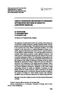
for the parameters. Thus, all final HRLS-PSO values are least squares regression estimates. After convergence of the swarms, the parameter values obtained were very close to the original values (see Col. 3 of Table I). Recovered parameters fit the simulated time course data as shown in Fig. IV. To check for the consistency of results, we performed 50 trials on the same data, differing only in the particle swarm optimizer random number generator initialization values. For input X6 = 15.0, the errors for the estimates were negligible except for four values (γ23 , γ33 , γ51 and f551 ) which nevertheless yielded small errors (3.85%, -3.89% ,-2.6% and 2.81% respectively). The largest parameter percentage errors were observed for input X6 = 6.0 which produced parameter domain errors of 167.39% -40.44% -14.77% -2.62% and 2.32% for γ23 , f233 , γ33 , γ51 and f551 respectively. Despite these large percentage values, the corresponding time domain errors for these parameters were negligible: 0.0086%, 0.00298%, 0.26%, 1.07%, and 0.5% respectively. The same trend was also observed for other input values. Thus, the profiles are insensitive to the values of these parameters. Convergence was always achieved and the standard deviations of the parameters from their mean values were very low.

to cut further the computation time in half. TABLE II C OMPUTATION T IME Equation 1 2 3 4 5 Total

min:secs 4:20 7:18 6:47 7:43 9:58 36:06

TABLE I AVERAGE PARAMETER E STIMATE P ERCENTAGE E RRORS FOR 50 RUNS OF P ROPOSED HRLS-PSO A LGORITHM ON S IMULATED Y EAST G LYCOLYSIS PATHWAY DATA . Param γ11 γ12 f121 f112 f152 γ22 f222 f252 γ23 f223 γ33 γ32 f332 f352 γ42 f432 f442 f452 γ51 f551

True Value 0.8122 196.129 -0.2344 0.7464 0.0243 16.5854 0.7318 -0.3941 0.012879 8.6107 9.59175 3.78146 0.6159 0.1308 325.08 0.05 0.533 -0.0822 25.1 1.0

Noise-free X6 = 15.0 0.00 0.01 0.00 0.00 0.00 0.00 -0.01 0.00 3.85 -0.43 -3.89 0.02 0.00 0.00 -0.04 0.17 -0.02 -0.04 -2.60 2.81

Noise-free X6 = 4.0 -0.01 -0.01 0.00 -0.01 0.00 -0.05 -0.05 -0.06 167.39 -40.44 -14.77 -0.01 0.00 0.00 0.03 -0.12 0.01 0.03 -2.62 2.32

Noisy Data σ = 0.10 -16.46 38.57 17.43 18.21 17.16 -12.49 17.08 13.60 336.26 -67.62 -97.95 -65.63 45.12 21.79 201.43 -98.34 57.68 114.92 -70.22 162.50

Fig. 1. Yeast Glycolysis Pathway Model time course profiles with parameters obtained from our proposed Hybrid Regularized Least SquaresParticle Swarm Optimization Algorithm exhibit close fitting with the data points used to train the algorithm.

One possible disadvantage of the use of the decoupling strategy is that it may be overly sensitive to noise in the derivatives. For this reason, the HRLS-PSO Algorithm was tested on noisy slopes. In this new set of experiments, the algorithmic settings were the same as for the noise-free case except for the population size which was doubled to 2000 particles. Gaussian noise was added to the concentrations and slopes at each time point: Xi (t)noisy = Xi (t)(1 + N (µ, σ 2 )) t ∈ [t0 , tN ]

The computation times for the five equations are listed in Table II. These values were obtained for a 3.0 GHz 64bit Intel Xeon Mac XServe. Overall computation time can still be reduced by exploiting the natural parallelism in the processing. Computations for the following pairs of equations can proceed independently of each other: equations 1 and 4; equations 3 and 5. With the availability of multicore processors, these independent computations can run in parallel as separate execution threads. With this scheme, it is possible

Si (t)noisy = Si (t)(1 + N (µ, (2σ)2 )) t ∈ [t0 , tN ] where N (µ, b2 ) denotes the normal distribution with mean µ and standard deviation b. Noise for slopes were four higher than those for concentrations since slope estimates could deviate as much as 2σ away from their true values [19]. Noisy datasets were generated with µ = 0.0 and noise levels σ = 0.02, 0.04, 0.06, 0.08, 0.10. HRLS-PSO results show that terms with one and two kinetic rate parameters tend to manifest quadratic dependence of parameter error

3700

with noise level.) We observe that terms with three kinetic rate parameters are much more sensitive to noise than those with fewer than three. The Glycolysis Pathway in Lactococcus lactis We now test the usefulness of the proposed algorithm on the extraction of rate constant and kinetic order parameters from actual experimental data. Neves et. al. [24] used nuclear magnetic resonance spectroscopy to study the sugar metabolism in Lactococcus lactis and their data which we use in our numerical experiments here was made available through [39]. The GMA Model equations for the simplified Glycolysis Pathway in L. lactis are as follows [39]: X˙ 1 X˙ 2

X˙ 3 X˙ 4

X˙ 5 X˙ 6 X˙ 7

= =

−β1 X1h11 X2h12 X5h25

α2 X1h11 X2h12 X5h25 − β2 X2h22 AT P h2,AT P

=

β2 X2h22 AT P h2,AT P − β3 X3h33 Pih3,Pi N ADh3,N AD

=

2β3 X3h33 Pi

=

h3,Pi

N ADh3 ,N AD + α4 X5g45 − β4 X4h44

β4 X4h44 − α2 X1h11 X2h12 X5h25 − α4 X5g45 hh51,P

−β51 X3h513 X5h515 Pi

i

− β52 X5h525

h51,Pi

= α2 X1h11 X2h12 X5h25 + β51 X3h513 X5h515 Pi

The swarms produced the parameter estimates listed in Table III. These values were close to those of [39] which were obtained manually and with considerable effort using a software tool called WebMetabol together with the user’s extensive knowledge of the domain. The logarithm of errors for each of the second to the sixth equations are (-9.914045, -5.915990, +2.41424, +1.531676, +3.025575) indicating good fits for the profiles of G6P and FBP and poor fits for the 3PGA, PEP and Pyruvate profiles. Time course data fit with GMA model for the six metabolites are shown in Fig. 2. Previous results obtained by Voit et. al. [39] are shown for comparison purposes. Substitution of the parameter values into the Glycolysis GMA Model with either kinetic orders h513 , h51,Pi or both equated to zero with the corresponding rescaling of the rate constant β51 yielded very similar predictions as the values of [39] thus validating our results. TABLE III PARAMETER E STIMATES FOR THE L ACTOCOCCUS LACTIS GMA M ODEL (PARAMETERS IN BOLDFACE WERE OBTAINED USING STANDARD L EAST S QUARES R EGRESSION )

−β61 X6h616 X3h613 N ADh61,N AD − β62 X6h626

Param α2 h11 h12 h25 β2 h22 h2,AT P β3 h33 h3,Pi α4 g45 h44

= β61 X6h616 X3h613 N ADh61,N AD

In this model, the key metabolites and enzymes are: Glucose (X1 ), Glucose-6-Phosphate (X2 ), Fructose Bi-Phosphate (X3 ), 3-Phosphoglycerate (X4 ), Phosphoenolpyruvate (X5 ), Pyruvate (X6 ), and Lactate (X7 ), ATP, NADH, inorganic Phosphate (Pi ). Time series data from in vivo NMR experiments of 13 C-labeled glucose in L. lactis were previously filtered using an artificial neural network and cubic splines. The slopes were subsequently computed using cubic splines using Matlab. The GMA differential equations above were decoupled, their left-hand side derivatives replaced with computed slopes and processed using the proposed algorithm with the following constraints: • Rate Parameters: (α2 , β2 , β3 , β52 ) ∈ [0.0, 100.0] (β51 , β52 , β62 ) ∈ [0.0, 10.0]; (α4 , β4 ) ∈ [0.0, 5.0] • Kinetic Parameters: (h33 , h3,Pi ) ∈ [−1.0, 0.0]; (h22 , h2,AT P , h44 , hh525 , h626 , h513 , h515 , g45 ) ∈ [0.0, 5.0]; h51,Pi ∈ [−5.0, 0.0] The HRLS-PSO settings used were the following: mutation probability = 0.5, population size = 1000, number of generations = 200, archive size = 500. Since the right hand side of the first and seventh differential equations are monomials with constant coefficients, they only require standard least squares computation and will therefore always converge to the same unique solution (see Table III values for β1 , h11 , h12 , h25 and β61 , h616 , h613 ). These parameter values were then used in the equations 2 and 6 which were computed next. The third and fifth equations both depend on the computational results of the second and sixth equations. Calculations for the fourth equation will wait for the results of the third and fifth equation before they could commence. Total computation time for this system was 41 min 8 secs.

Voit et al 0.3592 1.1287 -1.2906 0.2168 0.3115 2.1700 0.8152 0.4698 1.0297 0.2377 1.1452 3.5453 2.1649

HRL-PSO 0.287057 1.1287 -1.2906 0.2168 0.43412 1.973495 0.814113 0.475351 0.9918895 0.338727 1.015756 3.513723 2.087733

Param β51 h513 h515 h51,Pi β52 h525 β61 h616 h613 β62 h626 β4

Voit et al 0.9375 0.8744 0.0991 -0.0005 0.2087 0.0002 0.0417 0.6202 0.9263 1.3258 1.5255 2.1670

HRL-PSO 0.94035 0.868567 0.093747 -0.000487 0.204364 0.000201 0.0417 0.6202 0.9263 1.0792 1.51905 2.547663

V. C ONCLUSION In this paper, we have described a new hybrid parameter estimation algorithm for Generalized Mass Action (GMA) systems based on regularized least squares regression and multi-objective particle swarm optimization methods. Through a term-wise decomposition strategy in which the term parameters are estimated one term at a time, the algorithm circumvents the curse of dimensionality problem frequently faced by parameter estimation algorithms. Numerical experiments on simulated and actual experimental data show the effectiveness and accuracy of the algorithm. VI. ACKNOWLEDGEMENTS The authors would like to thank Prof. Eberhard O. Voit (Georgia Tech) for insightful comments and providing us the Lactococcus lactis dataset and Dr. Ricardo del Rosario (Max Planck Biochem and UP Diliman) for helpful discussions and suggestions.

3701

Fig. 2. Time-course plots for Lactococcus Lactis GMA model with parameters obtained from our proposed Hybrid Regularized Least Squares-

Fig. 3. Particle Swarm Optimization Algorithm. Previous estimates obtained by Voit et.al. [39] are plotted as dashed lines. Data are shown as dots.

3702

R EFERENCES [1] Almeida, J., and Voit, E.O. (2003). Neural-network based parameter estimation in complex biomedical systems. Genome Inform., 14,114– 23. [2] Bellman R.E. (1961). Adaptive Control Processes. Princeton University Press, Princeton, NJ. [3] Bj¨orkstr¨om, A. (2001). Ridge regression and inverse problems. Research Report in Mathematical Statistics, Stockholm University, 2000:5. [4] Chen, L., Bernard, O., Bastin, G., and Angelov, P. (2000). Hybrid modeling of biotechnological processes using neural networks. Control Eng. Pract., 8, 821–27. [5] Cho, DY., Kwang-Hyun, C., and Byoung-Tak Z. (2006). Identification of biochemical networks by s-tree based genetic programming. Bioinformatics, 22(13), 16 31–1640. [6] Chou, IC., Martens, H. and Voit, E.O. (2006). Parameter estimation in biochemical system models with alternating regression. Theor. Biol. Med. Model., 3(25). [7] Curto, R., Sorribas, A., and Cascante, M. (1995). Comparative characterization of the fermentation pathway of saccharomyces cerevisiae using biochemical systems theory and metabolic control analysis. model definition and nomenclature. Math. Biosci. 130,25–50. [8] Deb, K., Pratap, A., Agarwal, S., Meyarivan, T. (2002). A fast and elitest multiobjective genetic algorithm: NGSA-II. IEEE Trans. Evol. Comp. 6:2,182–197. [9] R. C.H. del Rosario, E. R. Mendoza, E. O. Voit. (2008). Challenges in Lin-log modeling of Glycolysis in Lactococcus lactis, IET Systems Biology 2:3, 136–149. [10] Eberhart, R and Kennedy, J. (1995). A new optimizer using particle swarm theory. Proc. 6th Int. Symp. Micro Machine and Human Science (MHS ’95), 39-43. [11] Gallazzo, J.L., and Bailey, J.E. (1990). Fermentation pathway kinetics and metabolic flux control in suspended and immobilized Saccharomyces cerevisiae. Enzyme Microb. Technol., 12, 162–72. [12] Gonzalez, O.R., K¨uper, C., Jung, K., Naval, P.C., Mendoza, E. (2007). Parameter estimation using simulated annealing for s-system models of biochemical networks. Bioinformatics, 23(4), 480–486. [13] Hansen, P.C. (1992). Analysis of ill-posed problems by means of the L-curve, SIAM Review, 34,561–80. [14] Ho, SY., Hsieh, CH., and Yu, FC. (2005). Inference of s-system models for large-scale genetic networks. InProc. 21st Int. Conference Data Engineering Workshops 2005, 1155. [15] Kikuchi, S., Tominaga, D., Arita, M., Takahashi, K., Tomita, M. (2003). Dynamic modeling of genetic networks using genetic algorithm and S-system. Bioinformatics, 19, 643–50. [16] Kim, KY., Cho, DY., and Byoung-Tak, Z. (2006). Multi-stage evolutionary algorithms for efficient identification of gene regulatory networks. LNCS 3907, Springer Verlag, 45–56. [17] Kimura, S., Ide, K., Kashihara, A., Kano, M., Hatakeyama, M., Masui, R., and Nakagawa, N. (2005). Inference of s-system models of genetic networks using a cooperative coevolutionary algorithm. Bioinformatics, 21, 1154–1163. [18] Kitayama, (2006). A simplified method for power-law modelling of metabolic pathways from time-course data and steady-state flux profiles.Theor. Biol. Med. Model., 3(24). [19] Kutalik, Z., Tucker, W., and Moulton, V. (2007). S-system parameter estimation for noisy metabolic profiles using newton-flow analysis IET Syst. Biol., 1:(3),174–180. [20] Lall, T., and Voit, E.O. (2005). Parameter estimation in modulated, unbranched reaction chains within biochemical systems. Comput. Biol. Chem., 29:,309–318. [21] Moles, C.G., Mendes, P., Banga, J.R. (2003). Parameter estimation in biochemical pathways: a comparison of global optimization methods. Genome Inform., 13:2467–2474. [22] Morosov, V.A. (1966). On the solution of functional equations by the method of regularization, Soviet. Math. Dokl., 7,414–17. [23] Noman, N. and Iba, H. (2005). Inference of gene regulatory networks using s-systems and differential evolution. In Proc. of Genetic and and Evolutionary Conference (GECCO 2005),439–46, ACM Press. [24] Neves, A.R., Ramos, A., Nunes, M.C., Kleerebezem, M., Hugenholtz, J., de Vos, W.M., Almeida, J.S., and Santos, H. (1999). In vivo nuclear magnetic resonance studies of glycolytic kinetics in Lactococcus lactis. Biotechnol. Bioeng., 64, 200–12.

[25] Polisetty, P.K., Voit, E.O., and Gatzke, E.P. (2006). Identification of metabolic system parameters using global optimization methods. Theor. Biol. Med. Model., 3(4). [26] Ramos, A., Neves, A.R., Santos, H. (2002). Metabolish of lactic acid bacteria studied by nuclear magnetic resonance. Antonie Van Leeuwenhoek 82 (1-4): 249-261. [27] Raquel, C.R. and Naval, P.C. (2005). An effective use of crowding distance in multiobjective particle swarm optimization. In Proc. of Genetic and and Evolutionary Conference (GECCO 2005),257–64, ACM Press. [28] Reyes-Sierra, M., and Coello Coello, C.A. (2006). Multi-objective particle swarm optimizers: A survey of the state-of-the-art. Int. J. Comp. Intel. Res.. 2(3), 287–308. [29] Seatzu, C. (2000). A fitting based method for parameter estimation in s-systems. Dynamic Systems and Applications, vol. 9, no. 1, 77-98. [30] Spieth, C., Streichert, F., Speer, N., and Zell, A.(2006). A memetic inference method for gene regulatory networks based on s-systems. In Proc. of IEEE Congress on Evolutionary Computation (CEC 2004),(1)152–157. [31] Spieth, C., Worzischek, R., and Streichert, F. (2006). Comparing evolutionary algorithms on the problem of network inference. In Proc. of Genetic and and Evolutionary Conference (GECCO 2006),279–286. [32] Tucker, W., Kutalik, Z., and Moulton, V. (2007). Estimating parameters for generalized mass action models using constraint propagation.Math. Biosciences,208(2): 607–620. [33] Ueda, T., Koga, N., and Okamoto, M. (2001). Efficient numerical optimization technique based on real-coded genetic algorithm Genome Inform., 12:451–453. [34] Voit E.O. (2000). Computational analysis of biochemical systems. Cambridge University Press, Cambridge, UK. [35] Vilela, M., Borges, C., Vasconcelos, A.T., Santos, H., Voit, E.O. and Almeida, J. (2007). Automated smoother for numeric decoupling of dynamic models. BMC Bioinformatics, 8:305. [36] Vilela, M., Chou I-C., Vinga S., Vasconcelos, A.T., Voit, E.O. and Almeida, J. (2008). Parameter Optimization in S-system models. BMC Syst. Biol., 2:35. [37] Voit, E.O. and Almeida, J. (2004). Decoupling dynamical systems for pathway identification from metabolic profiles. Bioinformatics, 20, 1670–81. [38] Voit, E.O. and Savageau, M.A. (1982). Power-law approach to modeling biological systems: III. Methods of analysis, J. Ferment. Technol., 60(3), 233–241. [39] Voit, E.O., Almeida, J., Marino, S., Lall, R., Goel, G., Neves, A.R. and Santos, H. (2006). Regulation of glycolysis in Lactococcus lactis: an unfinished system biological case study. IEE Proc. Syst. Biol., 153(4), 286–98. [40] Zitzler, E., Deb, K., and Thiele, L. (2000). Comparison of multiobjective evolutionary algorithms: empirical results. Evolutionary Computation, 8(2), 173–95.

3703