Partitioning Crowded Virtual Environments Anthony Steed, Roula Abou-Haidar Department of Computer Science, University College London Gower St, London, WC1E 6BT, United Kingdom
[email protected] ABSTRACT We investigate several techniques that partition a crowded virtual environment into regions that can be managed by separate servers or mapped onto different multicast groups. When constructing a partitioning, we attempt to minimize overhead of the partitioning with respect to network management, whilst maintaining a bound on the number of entities that are mapped to any particular server or group. We compare several partitioning schemes: quad tree, k-d tree unconstrained, k-d tree constrained, and region growing. With our simulations of a crowded virtual environment modelled on a part of central London, we find that the region growing technique give the best overall results.
Keywords Distributed virtual environments, spatial partitioning, multicast groups.
1 INTRODUCTION Collaborative virtual environments are becoming more popular especially for entertainment purposes. However the number of participants in an environment is often limited by the environment’s being supported by a single server. In this paper we investigate schemes that utilize usage data of a virtual environment in order to generate a static world partitioning so that multiple servers may be deployed effectively. Many researchers have looked at the problems of area of interest management and spatial partitioning (see Section 2). However these have mostly used regular partitionings of the virtual world. In this paper we ask a slightly different question: if we have a record or a prediction of aggregate behaviour of participants in a virtual world, how best can we plan to serve those participants in terms of minimizing participant, server and network costs? Using recorded activity data we build a partitioning using a topdown or bottom-up approach. We then analyze the effectiveness of the different partitioning strategies under different resource
requirements. The main requirement that we will try to meet is that servers must not get overloaded. If we can meet this requirement, then obviously we prefer schemes that require fewer servers. However we also note, as do Zou et al. [16], that there are significant run-time costs in the handover of a participant from one server to another. These may include the dynamic allocation of resources, resource reservation, routing changes and so on.
2 2.1
RELATED WORK Area of Interest Management
Although the single server/multiple client model of distributed virtual environments provides a well-understood and robust way of implementing today’s virtual environments (e.g. [12][13]), it has an obvious limitation in that the number of participants has to be capped to ensure stability. This capping is necessary due to the finite nature of server, client and network resources. The primary way in which scalability is achieved is to perform area of interest (AOI) management. An AOI management scheme considers the potential level of interest of each participant towards all other participants (e.g. [10]). Typical interest relationships might be, Participant A is interested in Participant B, if: • The distance from A to B is under some threshold, • A can see B, • A and B are performing similar tasks. There are embodiments of such schemes in many current collaborative virtual environment systems. There are many different ways of realizing such interest schemes. The ideal is to perform an exact partitioning with respect to the interest set, where the participant receives all and only those events that are of interest. However, if there are N participants there are O(N2) such potential interest relationships to consider and thus this calculation can become prohibitively expensive. Therefore implementations usually provide a conservative partitioning scheme where a super-set of the necessary events is delivered. For example, although a participant’s AOI rule might be that they are interested in all events that occur within a 5km geographical area, the underlying system might actually contain a hexagonal representation of space and the participant actually receive all events from all cells that overlap that 5km interest. The NPSNET system was based around such a mechanism [10].
space was partitioned into hexagonal cells, and each cell was associated with a multicast group. A participant would send data to the multicast group of the cell they were located in, but would receive data from all the multicast groups for the cells overlapping its AOI. Multiple server systems are an alternative. These place the responsibility for AOI management on a set of powerful servers that have good interconnections. With the RING system, Funkhouser has investigated two schemes [6]. The first allocates a server to a group of participants. The servers aggregate the AOIs of their clients, and inter-server communication is limited to the information necessary to satisfy the aggregate AOI. The second scheme allocates servers to regions of the environment. In this scheme, participants connect to the server that maintains the region they are interested in, and must switch servers when they reach the region boundary. Figure 1 Observed relative density of pedestrians around Regents St in central London (ObsWalkers). Areas coloured black are the most densely populated.
2.2
Spatial Partitions
The limitation of such regular partitionings is that since they are defined a priori, they don’t reflect how participants will actually use the space. Certain regions might be very crowded and thus they become failure points at run-time. A solution would be to locally refine the regular partition or add subregions at run-time. In [4], Farcet et al. analyze a dynamic octree partitioning scheme that adapts to the actual clustering of entities in the world. However maintaining world consistency with such a scheme would be difficult under real-world conditions. One limitation of AOI management as described so far, is that it is not reactive to load, but is an ideal relationship. Given that either the client, server or network still might suffer from overload, either the client AOI rules must adapt or the AOI resolution system must relieve the load by adding extra constraints, relaxing the satisfaction criteria by scaling regions of interest down, or in the worst case simply randomly dropping information. We call these approximate partitionings.
2.3
Network Architectures
The capabilities of an AOI management scheme are strongly tied to the network architecture underlying it. Although AOI management can be used on a single server to minimize network load and client load, once server load becomes the bottleneck, different architectures need to be investigated. Two primary architectures have been investigated in previous work: peer networks and multiple servers systems. A peer network certainly alleviates any server bottleneck, but now each client needs to perform an AOI interest calculation. Here in lies a catch: in order to make the AOI calculation it will need to know at least some information about all the other clients. In order to avoid this calculation becoming a bottleneck, one technique is to have a partitioning scheme that is built into the description of the environment, with this scheme mapping gross interest onto multicast groups. In the NPSNET system, the
Several variations on AOI management schemes can be found in the literature. The separation between logical AOI management and implementation is made concrete in Abram’s three-tiered architecture [1]. The MASSIVE systems have a very flexible AOI management system with dynamic adaptation of partitionings and high-level description of AOI relationships [3]. The Diamond Park system uses a beacon service to discover multicast regions [2]. The DIVE system places the multicast partitioning scheme under the control of a scripting language, making dynamic partitioning dependent on object behaviours as well as simple spatial partitions [7][5].
2.4
Cost of Partitioning
Any AOI management scheme that uses partitions suffers an overhead in the cost of managing that partition. For example, joining or leaving multicast groups is an operation that takes time and network resources. Switching servers similarly requires a potentially expensive re-allocation of network and server resources. In [16], Zou et al. phrase the partitioning problem as the minimization of inter-server transfers. They break down the environment into a coarse grid of N squares. They then build a simulation where there is a known likelihood of a participant transitioning between adjacent cells in the grid. From this they try to partition the space into a fixed number (M, where M < N) of server-managed regions, where the number of transitions of participants is minimized.
3
PROCESS OVERVIEW
From the discussion in Section 2, we believe that although spatial partitioning schemes have been widely discussed, implementations rarely take in to account how the space will actually be used. If a summary or prediction of usage patterns of a space is available, then we can attempt to optimize the partitioning scheme to generate a set of regions that will better satisfy future usage patterns. We have taken a hypothetical case based on pedestrian activity in a part of central London (see Figure 1). This is based on a real world monitoring of pedestrian flows along certain segments of pavement. It is an interesting data-set because it
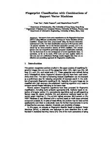
behaviour in the real world at the individual agent level is an open problem [11]. For these experiments we have used a very crude crowd model (see Section 5). This occasionally produces some un-natural behaviours, and agents in the simulation can get “stuck” for short periods in cycles within the map. Thus we have produced a second set of results, using a density map resulting from the simulated crowds (see Figure 2). We will refer to the observed and predicted data in Figure 1 as ObsWalkers, and to the simulated data in Figure 2 as SimWalkers. We have assumed that there will usually be a target number of participants for each server and that this is the same across all servers. The main cost of partitioning the space will then be in the handover between servers, and it is the number of handovers that needs to be minimized. We are not attempting to dynamically partition the world. Figure 2 Simulated pedestrian flows around Regents St in central London (SimWalkers). Areas coloured black are the most densely populated. has a large range of densities – many people walk up and down Regents St, but few make their way on to Brewer St. Unfortunately we do not have actual records of individuals’ behaviour. In the situation of an online game we might expect to have complete logs of player location over the lifetime of the game. The actual pedestrian data was limited in extent, so for our tests we augmented it with pavement and road information from UK Ordnance Survey databases by giving each unmonitored pavement and road a default pedestrian flow. Figure 1 illustrates the aggregate pedestrian as density ratios. Values of 0 (black) imply most dense, values of 1 (white) imply no occupancy. We can use this density map to make a region partitioning using a number of processes (see the following Section). However there is a limitation with this data – because we cannot track actual people in this space, we must build a simulation of pedestrian behaviour. Modelling of crowd
(a)
(b)
The process thus consists of the following steps: 1.
Creation of ObsWalker data
2.
Simulation of SimWalker data
3.
Partitioning of ObsWalker data with threshold T
4.
Testing of partitioning of ObsWalker with N agents
5.
Partitioning of SimWalker data with threshold T
6.
Testing of partitioning of SimWalker with N agents
Steps 3-6 are repeated for four partitioning schemes and different values of T and N. In Section 4 we discuss the partitioning schemes and in Section 6 we discuss strategies and experiments with varying T and N.
4 PARTIONING SCHEMES The crowd density maps are relative densities between 0 and 1. In this simulation we have used an 8-bit value and interpolated linearly between 0 and 1 for the density. We do not know the number of people in a crowd or the time-step of the simulation, and thus densities cannot be directly interpreted as an
(c)
(d)
Figure 3 Example partitionings of ObsWalkers. (a) Quad Tree partitioning giving 212 regions (b) K-D tree unconstrained partitioning giving 128 regions (c) K-D tree constrained partitioning giving 130 regions (d) Irregular region partitioning giving 162 regions
expectation that a particular cell will be occupied in a time period. To partition the model, we use a threshold value where the sum of the relative densities of a region should be less than the threshold. As we will see in Section 6, it is difficult to choose a threshold to achieve a particular constraint such as “in a simulation of X agents, no more than Y% of the time will more than Z agents be occupying any one server”. It is also difficult to predict the geometric properties that a good partitioning should have. Given a particular threshold constraint, if there are fewer regions in a partitioning, the average region density will closer to the target threshold. Obviously servers with a higher relative density have a greater probability of becoming overloaded. This must be traded off against the number of servers and the minimization of server handovers. At first glance this suggests that a partitioning where minimization of the total region boundary length might be an additional constraint. We have attempted to investigate these issues by experimentation and will discuss this further in Section 6. There are two main approaches to partitioning: top-down approaches that recursively split the world until regions satisfy the threshold constraint, and bottom-up approaches where regions are grown iteratively. The Quad Tree (Section 4.1) and both K-d Tree (Sections 4.2 and 4.3) algorithms are examples of top-down. The Region Growing (Section 4.4) is bottom-up.
4.1
Quad Tree
The first partitioning uses a quad-tree partitioning scheme. The relative density for a region is calculated, and if greater than the threshold the region is quartered and the process repeats. The algorithm is started by setting the initial region to the whole space. Figure 3(a) illustrates a partitioning on the ObsWalkers data with a threshold of 350 that generates 212 regions. In the figure the regions are coloured randomly for the purposes of illustration. For the quad tree and the k-d tree algorithms described below it is possible that after the partitioning some regions will have a relative density of zero. These are not counted and are removed from the simulation
4.2
K-d Tree Unconstrained
no roads following cardinal directions. Thus the K-d tree constrained algorithm additionally specifies that no region will have one edge longer than a given multiple of the other edge. This is implemented in the recursion by constraining the axis of the line of dissection and also the positioning of that line. This means that a particular split may not result in close to equal total relative densities in the two newly created regions. Figure 3(c) illustrates a partitioning on the ObsWalkers data with a threshold of 350 resulting in 130 regions. The allowed ratio of edge lengths in this example was 3. See [8] for a general analysis of K-d tree partitioning schemes.
4.4
Region Growing
The region growing technique is a variation of standard image processing algorithms for image partitioning. It starts from a seed point and adds adjacent points until a threshold is reached. The first naïve implementation uses a simple flood fill style algorithm. Once the threshold is reached, a new seed point is chosen. We prefer seed points that are close to the centre of mass of completed regions, and have high relative density. Due to the complex structure of the road system in this model, this results in very uneven distribution of region sizes, with many cells with small relative density. A revised algorithm grows regions until they are within a certain percentage of the threshold. A second pass then aggregates small regions onto larger adjacent regions. We have found that aiming for 90% of the threshold in the first pass gives good results. Figure 3(d) illustrates a partitioning on the ObsWalkers data with a threshold of 350 resulting in 162 regions.
5
CROWDING SIMULATIONS
We based our crowd simulation work on the system of Techia et al. [14][15]. This system can simulate and render crowds comprising 1000s of human figures at interactive frame rates. The first component of the system is an image-based rendering of virtual humans. The use of image-based rendering reduces the detail needed for a humanoid to one or two polygons with multiple textures. The second component is the simulation of crowd behaviour that uses a number of short-cuts in order to be able to achieve real-time performance.
This is another top-down algorithm. The relative density of a region is calculated and if it is greater than the threshold the region is dissected by a horizontal or vertical line. The line of dissection is chosen so that the two regions have as close to equal total relative density as possible. Splits are made alternately in the horizontal and vertical directions. The algorithm is started by setting the initial region to the bounding box of whole space. Figure 3(b) illustrates a partitioning on the ObsWalkers data with a threshold of 350 resulting in 128 regions. Note that there are many long, thin regions.
Each simulated humanoid, or agent, must collide with objects in the environment, avoid other agents and have a simple statemachine for navigation strategy. In the simulations run in this paper, agents have no high-level control. Later and separate versions of the system have incorporated agent strategies where the overall aggregate behaviour better correlates with actual observed behaviours [11]. Integration of more complex, perhaps non-real-time agent behaviours into our network simulations remains future work. Thus, as Section 6 will discuss, we have performed partitionings based on both observed and simulated crowd data.
4.3
Collision detection and avoidance are done using a discretisation of the space. In the system described in [14][15], a 2D collision map is extracted from the Z-buffer of a parallel projection rendering of the target model from a viewpoint above and looking straight down at the model. This collision map
K-d Tree Constrained
Very thin regions are potentially problematic when the aim is to minimize the number of handovers between regions. This is especially the case with the Regents Street data where there are
180 160 140 120 100 80 60 40 20 0
6 ANALYSIS
256
ObsWalker
212
128
130
120
SimWalker
232
128
129
143
Table 1 Region counts for the two data sets under different partitioning with threshold of 350 The base map measures 793x1023 pixels and 35% of the area is walkable in the ObsWalker data set. After the simulation we find that the agents reach each pixel in that map. The threshold relative density is 350. With the Quad Tree approaches we would expect that our smallest region would have 350/4 pixels. That is it resulted in a split of a region that was just above the threshold. Similarly for the K-d tree we would expect 350/2. Ideally with the Region Growing we would expect our minimum region size to be 350, but we will find smaller regions because of the difficulties in tiling together regions in a complex map. Figure 4 gives the region size frequency for each partitioning. The categories refer to a range of cell sizes, with each category covering double the range of the previous one. We can see that the constraint on region length imposed on Kd-Tree has little effect on neither number nor spread of region size.
84
2
6
8
0
16 3
Region Growing
50
81 9
K-d Tree Constrained
100
40 9
K-d Tree Unconstrained
150
20 4
Quad Tree
8192 16384
200
4
Figure 3 gave examples of partitioning to a given threshold for the ObsWalker data set. Table 1 shows the corresponding region counts for each partitioning method for both data sets.
4096
250
51 2
Partitioning Behaviour
2048
Cell size distribution in SimWalker partitioning with threshold of 350
25 6
6.1
1024
Cell size in range N to 2N-1
Number cells
There are three aspects to the analysis. Firstly we look at typical partitioning results for a fixed threshold and compare region counts and region sizes. Secondly we analyze a particular situation where the threshold is constant. We look at the four partitioning schemes, and investigate how they perform with both density maps. Thirdly we investigate how to tackle typical server reliability problems in more depth.
512
10 2
Note that our simulation is derived from the crowd system in [14], and does not support the advanced rendering and occlusion features of later systems [15].
Cell size distribution in ObsWalker partitioning with threshold of 350
Number cells
allows agents to walk over small steps. Since we only require planar movement, we can simply use the density maps as shown in Figures 1&2, and restrict agents to walking on nonwhite pixels. Collision between agents is avoided by each agent’s temporarily altering the 2D collision map to indicate the squares immediately adjacent to the square they are in are occupied. Thus, as agents move around the model they read and write collision information into this collision map.
Cell size in range N to 2N-1 Quad Tree
K-d Tree Unconstrained
K-d Tree Constrained
Region Growing
Figure 4 Cell size distributions for the two data sets with threshold of 350
6.2
Fixed Threshold Condition
Once the partitioning has been made, we run simulations to assess how many handovers between regions there are and to determine typical cell density patterns. Table 2 shows the number of handovers in a simulation with 1000 agents running over a 2000 step simulation period. The ranking of each partitioning is the same in each case, with Region Growing generating the smallest number of handovers. The difference between the best and worst is not that significant, being a matter of 20% or 10% difference. Notably, as was found in Table 1, the Quad Tree had many more cells than the others. The other techniques generated roughly the same number of cells on average.
Quad Tree
K-d Tree Unconstrained
K-d Tree Constrained
Region Growing
ObsWalker
19800
18938
17693
15766
SimWalker
20797
19188
18551
18145
Quad Tree
K-d Tree Unconstrained
K-d Tree Constrained
Region Growing
ObsWalker
99.1
97.9
97.8
95.2
SimWalker
99.8
99.2
99.3
99.3
Table 2 Handover counts for the two data sets under different partitionings with threshold of 350
Table 3 Percentage of server/time-steps with 16 or fewer agents
A more in-depth picture of what is happening is shown in Figure 5. This shows a summary across all servers and timesteps of how often a particular agent count was reached. We can see that the Quad Tree has fewer agents per cell as there are many more cells. The Region Growing technique has some cells with relatively few agents but the spread is also greater. The maximum number of agents in a cell was 30 in the Region Growing partitioning of the ObsWalkers data set. This happened 16 times over 120 regions, over 2000 time-steps (i.e. 0.0066% of the time).
Table 3 shows the percentage of servers/time-steps with 16 or fewer agents. This suggests that when the simulation does not fit the prediction (ObsWalker), Region Growing techniques gives a partitioning where regions have a higher likelihood of being congested. In this case on average 4.8% of servers were overloaded at any one time-step, whereas the Quad Tree, with roughly twice as many regions, gave an overload rate of only 0.9%. With the SimWalker data the K-d tree and Region growing algorithms perform roughly equally. In this situation the simulation behavior is following the density that was input into the partitioning.
6.3
Cumulative percentage of cells with a specific agent count (ObsWalker)
The previous two sections demonstrate the numbers of cells and number of handovers that can be expected. However, what is more pertinent when designing a real system is how many regions in each partitioning would be necessary to meet a particular reliability condition, and how many handovers would be produced?
Cumulative %
120 100 80 60 40
We will look at two scenarios using the ObsWalker data:
20
Agent count Cumulative percentage of cells with a specific agent count (SimWalker)
100 80 60 40 20
30
27
24
21
18
15
12
9
6
0 3
1000 participants are to be supported. The target server capacity is 16. A reliability of 95% is required
2.
4000 participants are to be supported. The target server capacity is 128. A reliability of 90% is required.
6.3.1
120
0
1. 30
27
24
21
18
15
12
9
6
3
0
0
Cumulative %
Reliability Target
Agent count Quad Tree
K-d Tree Unconstrained
K-d Tree Constrained
Region Growing
Figure 5 Server usages presented as cumulative percentage
Scenario 1
The use of the threshold is quite a crude device for selecting number of regions. We find that increasing the threshold from 330 through 410 in 8 steps does not change the number of KdTree regions with remained at roughly 128 regions. The Quad Tree does change size, but the total number of nodes remains high. At thresholds 330-410, each of these three algorithms performs in the range 97-99% reliability. At a threshold of 590 the number of cells in each of these methods has roughly halved (121, 64, 66 respectively), but the reliability of the Quad Tree remains high and the Kd-Tree algorithms have dropped below 90%.
Scenario 1: Occurence of 16 or fewer agents for various Region Growing partitionings in a 1000 agent simulation
Scenario 2: Region Counts for Thresholds 120
40 20
70
70
70
15
14
70
13
12
80 11
78
0
Threshold
80
0 0
85
10
0
60
0
90
98
50
80
88
95
Region Count
100
Reliability %
100
33 0 34 0 35 0 36 0 37 0 38 0 39 0 40 0 41 0
Numbers regions
100
150
Threshold
Reliability Percentage of servers with 128 or fewer agents under different partitionings
Figure 6 Graphs of reliability in Scenario 1
6.3.2
100 Percentage
80 60 40 20
7 DISCUSSION AND CONCLUSIONS We have examined the performance of four types of spatial partitioning in supporting large numbers of participants in a virtual environment. Specifically, we are trying to support more participants that can be allocated to a single server. We have taken as our case study, a hypothetical system that supports a number of participants visiting a virtual model of a part of central London. Because we do not have tracking data from individuals we have had to rely on a simulated crowd within this environment. However we did have some knowledge about the actual use of the real space by pedestrians and we incorporated that into a prediction of the use of space.
70
70
70
15
14
13
70 12
80
Threshold
Scenario 2
Figure 7 shows an analysis for Scenario 2. Again we see the features discussed in Section 6.3.1. The Quad Tree provides a range of regions sizes under the various thresholds. We see the drop in region count with the two K-d Tree algorithms. With the Kd-Tree algorithms we subsequently see a large drop in reliability. With the Region Growing technique we can select close to 90% reliability by taking a threshold of 980 giving 40 nodes. The best we can do with a Kd-Tree is a much better reliability of 98% with 62 nodes, and with the Quad-Tree algorithm, a reliability of 89.5% with 55 nodes. Again this shows the greater flexibility of Region Growing.
11
0
0
80 10
98
0
0 78
The Region Growing performs very differently producing different number of regions (see Figure 6). Lack of space prevents our including complete details, but we are able to get reliability close to 95% with a threshold of 360 producing 117 regions. During the simulation this generates 17340 region handovers. This compares well with the results for Quad Tree and Kd-Tree. Thus the Region Growing provides a lower number of handovers and lower number servers for the required reliability. The main observation is that Region Growing provides greater flexibility to meet different targets.
88
Regions
Quad Tree
K-d Tree Unconstrained
K-d Tree Constrained
Region Growing
Figure 7 Graphs of region count and reliability for Scenario 2
Throughout our analysis we compared the prediction of space usage with the usage of the space by the simulation. This reassures us that predicted usage forms a good basis for development of a spatial partitioning. However a shortcoming is that the crowd simulation model is not a good representation of actual human behaviour. We do not simulate the effects of points of interest in the model, nor temporal properties, such as commuting. In our model we have also assumed that virtual participants will walk with similar speeds and in the same places as real pedestrians. Of course, for proper application to a virtual world either real usage data will be needed or a better simulation model of participant behaviour. Our goal for the analysis was to investigate properties of the partitionings and also to attempt to find procedures for generating partitionings that could meet reliability criteria. The
first reliability criterion was a limit on the number of participants on a server. It is easy to generate partitionings that meet this criterion by creating many regions, but this both increases the number of servers or network groups that must be provisioned and increases the likelihood of a participant having to move between servers incurring significant run-time resources. Thus a partitioning must attempt to meet the participant limit but minimize the number of servers and the number of handovers. In Section 6 we found that a Region Growing technique can better satisfy the various requirements of a networked server system than a Quad Tree or K-d Tree based algorithm. We hypothesize that the Region Growing technique is better because, by the nature of the construction mechanism, it tends follows the likely connections between dense areas. In the other techniques, regions are rectangles and a single region might contain a number of disjoint navigable areas. For example, a region could contain two parallel streets where it isn’t possible to travel between the two streets without exiting the region. This means that, other things being equal, the likelihood that the participant will leave the cell within a short time period will be higher with these regular partitionings. Our usage of predicted models of behaviour as the basis for the ObsWalker data set was inspired by the analytic techniques of space syntax, where usage of space by pedestrians can be derived from analysis of configuration and connectivity of the real urban fabric [9]. In future work we hope to extend and apply such techniques to the prediction of usage of more abstract virtual worlds. Although the partitioning techniques have been developed for a London-based scenario, they are applicable to any type of environment. For more open environments, one of the regular partitioning schemes may as efficient as the Region Growing, but we expect that with environments with complex topologies of participant behaviour, an irregular partitioning such as Region Growing would prove superior. More complex worlds involving 3D structures would require different discretisations of space, but we would expect that the Region Growing strategy would still be productive across such discretisations. Finally, we have assumed a static partitioning scheme since it is easy to configure and it is reliable since the maintenance of the partitioning itself requires no server overhead or network traffic. However such a scheme will not work if participant numbers or usages of space change dramatically. If overall numbers or congestion in a particular region rises then regions could be dynamically split, but this re-introduces the problem of dynamically adding servers to a running system. However we have seen that a small subset of the servers might be relatively under-loaded so regions might dynamically created, but then allocated to currently under-utilized machines.
ACKNOWLEDGMENTS Thanks to Franco Tecchia, Celine Loscos and Yiorgos Chrysanthou for giving us access to their crowd simulation.
REFERENCES [1] H. Abrams, K. Watsen, and M. Zyda. Three Tiered Interest Management for Large-Scale Virtual Environments, Proceedings of VRST 98, 1998, Taipei. [2] J.W. Barrus, R.C. Waters, D.B. Anderson, Locales and Beacons: Efficient and Precise Support for Large MultiUser Virtual Environments, IEEE Virtual Reality Annual International Symposium, IEEE Computer Society Press, Los Alamitos CA, 1996. [3] S. Benford, C. Greenhalgh, D. Lloyd, Crowded Collaborative Virtual Environments, Proc. ACM CHI'97, Atlanta, US, March 1997, ACM Press. [4] N. Farcet, P. Torguet. Space-Scale Structure for Information Rejection in Large-Scale Distributed Virtual Environments, Proceedings of IEEE Virtual Reality Annual International Symposium, March 1998. [5] E. Frecon, G. Smith, A. Steed, M. Stenius, O. Stahl, An Overview of the COVEN Platform, Presence: Teleoperators and Virtual Environments, 10(1), February 2001, pp. 109-127 , MIT Press, ISSN 1054-7460 [6] T.A. Funkhouser, Network Topologies for Scalable MultiUser Virtual Environments, IEEE VRAIS `96, San Jose, CA, April, 1996. [7] O. Hagsand, Interactive Multiuser VEs in the DIVE System. IEEE Multimedia, Spring 1996, Vol. 3, No.1, pp. 30-39, IEEE Computer Society, ISSN 1070-986X [8] V. Havran, Heuristic Ray Shooting Algorithms, PhD Thesis, Czech Technical University, Prague, 2000. [9] B. Hillier, Space is the Machine, Cambridge University Press, 1996, [10] M.R. Macedonia, M.J. Zyda, D.R. Pratt, D.P. Brutzman, P.T. Barham, Exploiting Reality with Multicast Groups, IEEE Virtual Reality Annual International Symposium, (VRAIS’95). September 1995, pp.38-45. [11] A. Turner, A. Penn, Encoding natural movement as an agent-based system: an investigation into human pedestrian behaviour in the built environment. Environment and Planning B: Planning and Design 29:473-490 [12] S. Sandeep, M. Zyda, Networked Virtual Environments Design and Implementation, ACM Press Books, SIGGRAPH Series, 23 July 1999, ISBN 0-201-32557-8 [13] D. Snowdon, C. Greenhalgh, S. Benford, A. Bullock, C. Brown, A Review of Distributed Architectures for Networked Virtual Reality, Virtual Reality: Research, Development and Applications, Vol. 2 No. 1 1996. [14] F. Tecchia, C. Loscos, Y. Chrysanthou, Real Time Rendering of Populated Urban Environments, ACM Siggraph'01 technical sketch, Los Angeles, California, USA, August 2001. [15] F. Tecchia, C. Loscos, Y. Chrysanthou, Image Based Crowd Rendering, IEEE Computer Graphics and Applications, March/April 2002 (Vol. 22, No. 2). [16] L. Zou, M. Ammar, C. Diot. An Evaluation of Grouping Techniques for State Dissemination in Networked MultiUser Games. Proceedings of the Ninth International Symposium on Modelling, Analysis, and Simulation of Computer and Telecommunication Systems, (MASCOTS'01), August 2001.