Probabilistic Modeling and Recognition of 3-D Objects - Pattern ...

International Journal of Computer Vision 39(3), 229–251, 2000 c 2000 Kluwer Academic Publishers. Manufactured in The Netherlands. !

Probabilistic Modeling and Recognition of 3-D Objects JOACHIM HORNEGGER AND HEINRICH NIEMANN Lehrstuhl für Mustererkennung (Informatik 5), Universität Erlangen–Nürnberg, Martensstr. 3, 91058 Erlangen, Germany [email protected] [email protected]

Received January 30, 1998; Revised December 13, 1999; Accepted June 19, 2000

Abstract. This paper introduces a uniform statistical framework for both 3-D and 2-D object recognition using intensity images as input data. The theoretical part provides a mathematical tool for stochastic modeling. The algorithmic part introduces methods for automatic model generation, localization, and recognition of objects. 2-D images are used for learning the statistical appearance of 3-D objects; both the depth information and the matching between image and model features are missing for model generation. The implied incomplete data estimation problem is solved by the Expectation Maximization algorithm. This leads to a novel class of algorithms for automatic model generation from projections. The estimation of pose parameters corresponds to a non-linear maximum likelihood estimation problem which is solved by a global optimization procedure. Classification is done by the Bayesian decision rule. This work includes the experimental evaluation of the various facets of the presented approach. An empirical evaluation of learning algorithms and the comparison of different pose estimation algorithms show the feasibility of the proposed probabilistic framework. Keywords: statistical object recognition, pose estimation, expectation maximization algorithm, mixture densities, hidden Markov models, marginalization, global optimization, adaptive random search

1.

Introduction

The research field computer vision summarizes a wide range of problems from low-level image processing, 3-D reconstruction, surface approximation, object tracking to object identification and pose estimation (Trucco and Verri, 1998). A major problem and still unsolved task is the automatic learning, localization, and recognition of 3-D objects from intensity images. Generally, a recognition system is expected to identify and locate arbitrary objects of a model database in complex scenes, even with cluttered background and under varying illumination conditions. The involved algorithms should have no limitations to special types of objects or any constraints for viewing directions. The application of statistical methods to tackle the problem of learning, localizing, and recognizing objects is becoming more and more popular. There is some hope that the combination of geometry and

statistics will allow the development of a new generation of vision algorithms which will improve currently known and applied methods (Kanatani, 1996). This work extends the probabilistic framework for object recognition originally introduced by Wells (1997). We describe an optimal way (at least from a theoretical point of view) to deal with common problems in 3-D object recognition. The developed concepts provide a model-based statistical recognition system which allows

! automatic learning, ! identification, and ! pose estimation.

The mathematical framework treats the correspondence problem, relational dependencies between features, as well as segmentation errors in a uniform probabilistic manner. Furthermore, the proposed theory

230

Hornegger and Niemann

allows 2-D as well as 3-D object recognition. We use image features for recognition and for pose estimation that range from point features to line features and we include the relational dependencies between them. 1.1.

Model-Based Object Recognition

Model-based approaches represent the state-of-the-art techniques to solve the object recognition and localization problem (Jain and Flynn, 1993; Ponce et al., 1996; Trucco and Verri, 1998). Implementations of modelbased recognition and pose estimation algorithms differ from each other with respect to the representation of models, the method for the comparison of computed image features and model data, and the judgment of hypothesized object classes and pose parameters. Object models and the projection, which maps features from 3-D to 2-D, have to provide all the information required for recognition and pose estimation. Depending on the image features used and the strategy selected for classification, there exists a wide range of different approaches to object modeling (Ponce et al., 1996). All of them should provide descriptions which are unambiguous, unique, convenient to use, and non-sensitive to noise or segmentation errors (Jain and Flynn, 1993; Faugeras, 1993; Horn, 1986). In this paper observations are considered as random measures and models are defined by probability density functions. 1.2.

Motivation for a Statistical Approach

In the following, our objective is the construction of a probabilistic object recognition system which fits all the basic requirements of model-based vision systems. An obvious and crucial question is, why we should prefer statistical methods to commonly used recognition algorithms. It is important to comment on this because there already exists a broad field of well studied and quite powerful modeling techniques and recognition algorithms. Most of these approaches are based on pure geometry and the application of distance measures for decision making (Jain and Flynn, 1993; Ponce et al., 1996). Indeed, there are several fundamental, both theoretical and practical, arguments which suggest the use of probabilistic principles for computer vision purposes. The most important arguments are as follows: 1. Probabilistic methods are successfully applied and state-of-the-art techniques in pattern recognition (Bishop, 1995; Ripley, 1996). The success of speech recognition systems, for instance, is essentially based on statistical methods (Jelinek, 1998).

Probabilistic models facilitated the commercial use of speech recognition systems. 2. Images and segmentation results (used both for model generation and classification) are not stable. There are changes due to illumination, sensor noise, and variations in pose. Segmentation results vary considerably. An adequate mathematical description is needed which incorporates these properties. We should consider a statistical approach because this framework is especially designed to deal with uncertainties and randomized processes. 3. Parameter estimation techniques from mathematical statistics or non-parametric estimation methods can be applied to model generation (McLachlan and Krishnan, 1996). The available mathematical results will support and simplify the development of algorithms. 4. A well-known theorem from decision theory states the optimality of Bayesian classifiers with respect to misclassification rates (Bishop, 1995; Ripley, 1996). 1.3.

Addressed Problems

As it is implemented by the theoretical result on Bayesian classifiers, the ultimate goal of all classification systems should be the close approximation of the Bayesian decision rule. This is claimed easily. But the concrete construction of statistical object models appropriate for solving the 3-D object recognition problem using 2-D projections is neither obvious nor nontrivial. It is still an open problem whether statistical methods allow to model the real world sufficiently for computer vision purposes. For the implementation of a probabilistic recognition system the following six practical problems have to be addressed and will guide the remainder paper: 1. object modeling: An adequate, discriminative statistical model has to be constructed within the chosen probabilistic context. We have to provide either a discrete probability distribution or a continuous probability density function (p.d.f). 2. model learning: Training algorithms are required for the automatic estimation of model densities. Manual interaction should be avoided. 3. statistical inference: Efficient algorithms are needed for the statistical judgment of observed features and relational dependencies. 4. matching: Recognition usually demands methods for the computation of correspondences between image and model primitives.

3-D Objects

5. pose estimation: Pose estimation has to be computationally efficient and robust. 6. classification: Classification should apply the Bayesian decision rule. Partial solutions to these problems were already discussed in the literature. Especially in Wells (1997) the 2-D object recognition problem using 2-D image data is nearly completely treated; however, this approach is restricted to 2-D point features; the important step of automatic model learning is missing as well as the problem of modeling 3-D objects and their appearance in 2-D. The incorparation of projection models as well as intrinsic and extrinsic sensor parameters is also part of our extended probilistic modeling scheme. Therefore we contribute some novel ideas to this existing approach. We provide a complete probabilistic framework which satisfies the above mentioned requirements for 3-D object learning, pose estimation, and recognition from 2-D views. We make extensive use of the Expectation Maximization algorithm, of independency assumptions to beat the curse of dimensionality, and of marginals to reduce and to decompose high dimensional search spaces. 2.

Related Work

The use of statistical methods for image processing and computer vision purposes has a long tradition. Statistics can be found in many vision systems from low- to high-level applications (Hornegger et al., 1999; Wells, 1997; Winkler, 1995). Fields of most practical relevance range from image and texture modeling (Zhu et al., 1998), image filtering and restoration (Winkler, 1995) to recognition and pose estimation Wells (1997). The results on probabilistic 2-D recognition and localization achieved in Wells (1997) as well as the success of hidden Markov models in speech recognition and analysis motivated our research on probabilistic 3-D vision. The object recognition process and its complexity are (up to these days) crucially related to the model and the matching strategy of image and model features. The recognition algorithm has to be robust with respect to possible mismatching decisions. Statistical approaches which deal with these types of problems are already in use. Examples can be found in Pope (1995) and Wells (1993). Solely pairwise statistically independent assignments are assumed there. Like in hidden Markov modeling, Wells suggests modeling the assignment as

231

a random process independent of the spatial distribution of features; point features and their statististical properties are separated from the assignment; they are assumed to be normally distributed. In the final p.d.f the unknown assignment is eliminated simply by marginalization. Therefore the associated algorithms do not require feature matching. The final estimation of 2-D orientation and translation can be done without considering feature correspondences.In contrast to this approach, the matching problem might also be considered as a labeling process. Statistical dependencies are explicitly computed by probabilistic relaxation methods as suggested in Kittler et al. (1993). Our work picks up the probabilistic modeling of the assignment function as described in Wells (1993) and extends it to a more general probabilistic setting including dependencies of higher order and the incorporation of neighborhood relations. Within a probabilistic framework,the recognition of objects is easily done by applying the Bayesian decision rule, even in the presence of incomplete knowledge (Dubuisson and Masson, 1993). The same holds for the classification module of this work. Statistical models of objects and the observed features are used for computing the posterior probabilities. The pose estimation problem is considered in different manners in the literature: some authors use view based approaches to 3-D object recognition (Wells, 1993). There, localization corresponds to the computation of the correct 2-D view. Pose estimation is considered as a 2-D classification process (Trucco and Verri, 1998), and the precision of pose parameters depends on the quantization of the viewing sphere.The interpolation of 2-D views can be applied for refinement (Ullman, 1996). Other authors use various types of 3-D models and reduce the pose estimation problem to an optimization task (Cagliotti, 1994). They apply CAD-models for localization (Ponce et al., 1996) or utilize precomputed statistical 3-D models using line features and related measures (Kanatani, 1993; Trucco and Verri, 1998). Also the EM algorithm proves to be suitable for pose estimation of 2-D objects, but it requires an appropriate initialization close to the global maximum of the chosen objective function (Wells, 1993). For that reason, we propose the use of global optimization techniques based on adaptive random search methods. Pose estimation here is not restricted to 2-D object recognition. It also allows for 3-D localization and classification using gray-level images. The preceding discussion shows that the use of statistical methods regarding several components of

232


vision systems are well elaborated. Complete solutions, however, which represent an entire statistical object classifier, and treat model generation, localization, and classification, are rather the exceptional case (Hornegger et al., 1999; Murase and Nayar, 1995; Pope, 1995; Schiele, 1997). 3.

Statistical Object Recognition

This section introduces the basic notation and formalism required for the subsequent derivations and descriptions of algorithms. 3.1.

Rigid Objects

We restrict the discussion to rigid objects. Two objects are defined to be elements of the same object class, if their geometrical 3-D structure is equal. There is no distinction between objects of identical shape and different colors. Only geometry defines pattern classes. In the following, we consider K different object classes which are denoted by !κ , κ = {1, 2, . . . , K }. Two objects are of the same class, if the observed image or a subset of observed features is assigned to the same object class !κ . Classification and pose estimation require models which characterize object classes and allow the computation of similarity measures between observed image features and the object model. Obviously, if features vary with the position and orientation of the considered object, the similarity measure will depend on pose parameters. 3.2.

Features and Assignments

Statistical classifiers require probabilistic models. Each object class has to be represented by a p.d.f. Its arguments are random measures computed from the given sensor data. Generally, we distinguish between two different types of features: 2-D and 3-D. The type of the feature depends on the space in which the object is considered. An observed 2-D corner in the image, for example, has a corresponding 3-D corner of the object. Therefore, we call the 2-D features computed from sensor data image features and 3-D features corresponding to objects in 3-D model features. Image features are transformed model features mixed with additional background features and corrupted by segmentation errors.The set of model features belonging to object class !κ is denoted by Cκ = {cκ,1 , cκ,2 , . . . , cκ,n κ }. These features belong to the model space and their dimension is Dm . The Do -dimensional image space yields the set of image features O = {o1 , o2 , . . . , om }.

It is obvious that an object in the image plane cannot be represented by a single feature vector or a set with a fixed number of vectors. A set of possibly related and mutually dependent features is required to characterize an object. There is also the need for the assignment of image and model features, and the registration of relational dependency structures. A statistical object recognition system has to provide techniques for describing the matching procedure (c.f. (Wells, 1993)) and the relations between features in a statistical manner. Example. If we work on 3-D object recognition problems using gray-level images and point features O = {o1 , o2 , . . . , om }, we have three-dimensional model points cκ,l ∈ R3 and two-dimensional observations ok ∈ R2 . In this case Dm = 3 and Do = 2. The matching problem is the assignment of the segmentation result (the 2-D points) to features of a model κ from the model data base. The assignment of observed features ok (1 ≤ k ≤ m) to model features cκ,l (1 ≤ l ≤ n κ ) is unknown. A possible relational dependency might be a neighborhood relationship of point features (e.g., two points are connected by a line) or visibility constraints (e.g., mutual occlusion). 3.3.

Bayesian Classifier

Recognition of an object corresponds to a classification problem. In pattern recognition theory, statistical classifiers expect the complete statistical knowledge of the problem domain. For a model feature c ∈ R Dm of prior known and fixed dimension Dm , the parametric probability density function p(c; aκ ) must be given, where c belongs to an object of class !κ , and aκ denotes the class-specific parameter of the density; again the number of considered classes is K , i.e. 1 ≤ κ ≤ K . In addition, the prior probability p(!κ ) for each class !κ is required because the decision is based on the maximization of the a posteriori probabilities p(!κ | c). The Bayesian classifier applies the following decision rule λ = argmax p(!κ | c) = argmax κ

κ

p(!κ ) p(c; aκ ) . p(c) (1)

There is no straightforward application of this decision rule to solve object recognition problems for two reasons:

! the statistical description of 3-D objects observed in

2-D images is generally not possible using one single feature vector, and

3-D Objects

! due to segmentation errors and occlusion the number of image features is not constant.

The computation of a unique, bijective mapping of image to model features is, in general, impossible. Obviously we need p.d.f.’s which allow the computation of a density value for observed image feature sets of variable cardinality. 3.4.

Incorporated Feature Transform

Not only the size of image feature sets varies with different views, but also the position of features and their relationship in the image plane. Features depend on the camera and the object position in the chosen world coordinate system. Therefore, the projection into the image plane as well as rotation and translation of objects should be part of statistical models and considered during the decision process. In Wells (1997) the author suggests transforming the observed features in the image plane instead of incorporating the transform to the p.d.f. This is sufficient for 2-D recognition where we have only planar rotations and translations and no projection. In case of observing 3-D objects in the 2-D image this strategy is no longer applicable. The p.d.f. has to be parameterized with respect to the transformation, including 3-D rotation, 3-D translation and the projection mapping. If image features change with the object’s pose, parameters of the density function are necessary which characterize the rotation and translation defined by a bijective affine mapping R ∈ R Dm ×Dm and t ∈ R Dm . Thus, the density for each transformed feature c% = Rc + t ∈ R Dm will include two different types of parameters: object- and pose-specific parameters. This is quite similar to the notion of extrinsic and intrinsic parameters known from camera calibration. The parametric density is p(c% ; aκ , R, t), where aκ denotes the object-specific and R and t the pose-specific parameters. The incorporation of pose-specific parameters into a single density p(c; aκ ) can be done by a standard density transformation (Anderson, 1958). The same holds for the embedding of the projection model. The density of the projected image features o ∈ R Do results from a density transform and a subsequent marginalization over the random variables lost by projection. The extended Bayesian decision rule using densities with incorporated feature transforms obviously is λ = argmax p(!κ | o) = argmax κ

κ

p(!κ ) p(o; aκ , R, t) . p(o) (2)

233

Considering decision rule (2) we conclude that in addition to aκ , pose parameters R and t have to be known for object classification. Example. Let us assume a normally distributed 3-D point feature c ∈ R3 of the 3-D model space with mean vector µκ ∈ R3 and the symmetric, positive semidefinite covariance matrix Σκ ∈ R3×3 . This point is rotated and translated in the model space, and projected into the 2-D image space by orthographic projection. The parametric probability density function of the 3-D model feature c is given by p(c; aκ ) = N (c; µκ , Σκ ) ! " exp − 12 (c − µκ )T Σ−1 κ (c − µκ ) . (3) = √ det (2π Σκ ) In this example, the parameter aκ of the above introduced notation includes in this example simply the mean vector and the covariance matrix. There exist different representation methods for 3-D rotations (Altmann, 1986). For instance, a rotation in the model space can be defined by a (3 × 3)-matrix R = Rx R y Rz . The rotation matrix depends on the Euler angles φx , φ y , and φz , the rotation angles around the x-, y-, and z-axis of the world coordinate system. A translation of model features is defined by a vector t = (t1 , t2 , t3 )T ∈ R3 . The complete mapping given by R and t has six degrees of freedom. The pose estimation is restricted to the robust estimation of these parameters. Due to the affine nature of this transform, the density of rotated and translated normally distributed model features c% = (c1% , c2% , c3% )T ∈ R3 is again Gaussian. The mean vector is Rµκ +t and covariance matrix results in RΣκ RT (Anderson, 1958). This result holds even for arbitrary affine transformations from the model into the image space, as long as Dm ≥ Do . The density of the projected image feature o ∈ R2 is given by the marginal density p(o; aκ , R, t) =

#

p(c% ; aκ , R, t) dc3% ,

(4)

where the lost range component c3% is integrated out. Since an orthographic projection can be described by an affine mapping, the resulting distribution (4) of the observed, projected image feature is also Gaussian. If model- and pose-specific parameters are known,we can evaluate the density (4) for arbitrary image features and get a statistical measure for their probability.

234


3.5.

Probabilistic Formalization of Addressed Problems

The construction of appropriate densities and the implementation of each stage are the major concerns of the upcoming sections.

So far the discussion allows an abstract description of the major components of statistical object recognition systems ignoring mathematical details of the densities’ structure. The set of observed image features is given by O = {o1 , o2 , . . . , om }. Let p(O; Bκ , R, t) be the probability density function with incorporated feature transform corresponding to object class !κ for the set O of appearing features. Here Bκ summarizes all object-specific parameters, whereas R and t symbolize the transformation parameters in the model space. The projection model is assumed to be known and implicitly implemented in p(O; Bκ , R, t). Densities describing objects and their statistical behavior in the image plane are called model densities. Using these model densities, we conclude that both the model generation process and the localization of known objects correspond to parameter estimation problems. These can be solved by maximum likelihood estimation, and we denote the estimate of a parameter by a “ ˆ ”. The classification, however, uses the Bayesian decision rule (2). The stages required for a statistical object recognition system are formally characterized by:

! object modeling which is the concrete representation

! model learning which corresponds to the parameter of the p.d.f. p(O; Bκ , R, t). estimation problem ˆ κ = argmax B Bκ

N $

log p(& O; Bκ , & R, & t),

(5)

4.

Construction of Model Densities

This section introduces the concrete structure of probabilistic models which are used to build a 3-D recognition and pose estimation system. The concept distinguishes between different types of random processes, and between hidden and observable random variables. Marginalization proves to be an extremely powerful mechanism for the elimination of hidden random variables. A final composed probability density function is used to derive various statistical models by specialization and by introducing independency assumptions. It is shown how this class of density functions is related to well-known statistical models, like mixture densities or hidden Markov models. We also suggest further generalizations of well established standard modeling schemes (Jelinek, 1998; Li et al., 2000). 4.1.

Model Densities

We start with the introduction of a probabilistic model which allows the probabilistic description of image features and of relations among image features. Model densities, which are suitable for various types of pattern recognition problems, can be constructed by looking at the involved components (e.g., assignment of image and model features, rotation, translation, projection, etc.) in detail.

&=1

for a given set of N training views which differ in image features {& O | 1 ≤ & ≤ N } and in the associated set of pose parameters {& R, & t | 1 ≤ & ≤ N }; ! statistical inference which requires the efficient evaluation of the p.d.f. p(O; Bκ , R, t) in the absence of explicitly matched features; ! matching which is the explicit computation of correspondences between image and model features; ! pose estimation formalized as the global optimization task ˆ ˆt} = argmax p(O; Bκ , R, t), {R,

(6)

R,t

for a given class κ,where the image features O of a single view are used for object localization; ! classification applying Bayes decision rule which requires the priors of classes and the p.d.f. associated with each class.

4.1.1. Probabilistic Modeling of Image Feature Sets. In Section 3.4 the statistical modeling of single model and image features using simple density functions with an incorporated feature transform was introduced (c.f. (3) and (4)). If observed image features of fixed dimension are transformed model features and if the class of parametric transformations is known, the original density functions p(c; aκ,l ) (1 ≤ κ ≤ n κ ) of model features can be extended with respect to pose-specific parameters and result in densities for corresponding image features p(o; aκ,l , R, t) (c.f. Section 3.4). Given the assumption that the densities of all image features are known, the probabilistic characterization of a set of image features O = {o1 , o2 , . . . , om } is given by the product of single density functions. Herein, the observations are assumed to be pairwise statistically independent. If the corresponding pairs (defined by the assignment function ζκ , c.f. Section 4.1.2) of image and

3-D Objects

with each image feature set O a discrete random vector

model features are known, we get p(O | ζ κ ; Bκ , R, t) =

m % k=1

p(ok ; aκ,lk , R, t).

(7)

This model density relates image features O and model features Cκ , if the corresponding pairs of image features ok and model features cκ,lk are known and if the pose parameters R and t are given. Since our objective is the probabilistic description of the complete objects and their appearance in the image plane, the statistical modeling of the assignment function ζκ is required. 4.1.2. Probabilistic Modeling of Feature Correspondences. The probabilistic modeling of the assignment function, which relates image and model features, enforces the introduction of a discrete random process. Therefore, we introduce according to Wells (1997) the assignment function ζκ between the set of image features O = {o1 , o2 , . . . , om } and model features Cκ = {cκ,1 , cκ,2 , . . . , cκ,n κ } using the definition ζκ :

&

O → {1, . . . , n κ } ok *→ lk, k = 1, 2, . . . , m.

(8)

Herein, ζκ maps the observed image feature ok to the index lk of its corresponding model feature cκ,lk . For simplicity, we assume that all image features have a corresponding model feature, i.e. ζκ is a total mapping. Due to occlusion and segmentation errors, not all model features have corresponding image features. Segmentation errors might also mean that one model feature can have more associated image features. For that reason, ζκ is neither injective nor surjective. One single image feature cannot correspond to more than one model feature. The mapping ζκ defines a function and in real image data two different model features should not generate identical image features. The introduction of the assignment function ζκ now allows a statistical formalization of the assignment between image and model features. We simply associate

Figure 1.

Matching of image and model features.

235

ζ κ = (ζκ (o1 ) . . . , ζκ (om ), )T

= (l1 , . . . , lm , )T ∈ {1, . . . , n κ }m .

(9)

This random vector ζ κ is attached to a discrete probability p(ζ κ ), which results in a probabilistic measure for assignment functions and given sets of image features. For each assignment function the probability for its occurrence can be computed. Given that assignments are considered ' as random measures the probability constraint ζκ p(ζ κ ) = 1 is valid. On the one hand the advantage of the probabilistic characterization of assignments is that we have a statistical measure for each considered matching. On the other hand statistical modeling permits the use of marginals and the elimination of random variables of multivariate density functions (Jelinek, 1998; Wells, 1997), i.e. also the elemination of assignments. Example. Figure 1 shows an example of a discrete assignment function, symbolized by arrows. The gray colored ellipse illustrates the loss of information during the projection θκ from the model into the image space.The resulting random vector for this example is ζ κ = (1, 3, 2, 2, 5, 6, 6, 5)T . 4.1.3. Probabilistic Modeling of Relations. The basic idea for statistical modeling of assignment functions is the introduction of a discrete random vector and the embedding of this random vector in a measure space. This procedure can also be applied for the statistical modeling of relational dependencies between features. An arbitrary q-ary relation of image features is defined by the indicator function & 1, if the relation is satisfied " ! . χ ok 1 , . . . , o k q = 0, otherwise (10)

Using this definition for each q-tuple (ok1 , . . . , okq ) of observed features, we get a Boolean value, which indicates, whether the tuple satisfies the relation or not.

236


The q-ary relation and the associated Boolean values induce a random array ν = (νk1 ,...,kq )1≤k1 ,...,kq ≤m

ζκ and the Boolean matrix ν ∈ Rq×q results from the components introduced so far. The joint probability function

(11)

p(O, ν, ζ κ ; Bκ , R, t)

The entries of this array show a randomized behavior. Due to segmentation errors and variations within the sensor data, the observable relations in the image plane are not deterministic. In accordance with the statistical modeling of the assignment function, we relate this matrix to a conditional discrete probability p(ν | ζ κ ), where +ν p(ν | ζ κ ) = 1. The probability of the random array depends on the assignment ζκ of image and model features. Observable relations are usually induced by dependencies in the model space.

= p(ζ κ ) p(ν | ζ κ )

= (χ(ok1 , . . . , okq ))1≤k1 ,...,kq ≤m .

Example. A concrete example for relational dependencies yields the neighborhood relationship between image features. Two image points, for instance, are said to be neighbors, if they are connected by a line.In Fig. 2 (middle), for example, o1 and o2 are neighbors, whereas o2 and o3 are not. The aleatory matrix for the complete segmentation result (Fig. 2, middle) is   0 1 0 1 1 0 0   1 0 0 0 0 1 0   0 0 0 1 0 0 1     (νk % ,k %% )1≤k % ,k %% ≤7 = 1 0 1 0 0 0 0 . (12)   1 0 0 0 0 1 0     0 1 0 0 1 0 1 0 0 1 0 0 1 0 Due to the fact that the neighborhood relation is symmetric, this indicator matrix ν is symmetric. 4.1.4. Probabilistic Modeling using Joint Density Functions. The joint density for observing a set of m image features O with a given assignment function

Figure 2.

m % ! " p ok ; aκ,ζκ (ok ) , R, t . (13) k=1

combines the continuous density function (7) for image features with the discrete probabilities for the assignment function and the observed relations. This model density allows the computation of statistical measures for observations. These include the features and relations. The assignment function ζκ is usually not part of the observation. The model density (13) seems inappropriate because it requires the knowledge of the latent assignment ζκ . An obvious way to deal with this problem is search for an optimal match. All assignments are judged by (13), and we decide for that matching with highest density values. However, if the computed assignment function is wrong, this would affect subsequent processing steps like localization and classification. Fortunately the statistical modeling of the assignment process allows for a more powerful technique: the marginalization (Jelinek, 1998; Wells, 1997). We eliminate the unknown matching by summation over all possible assignments instead of solving a discrete search problem to find the best match. The marginal density results in p(O, ν; Bκ , R, t) $ p(O, ν, ζ κ ; Bκ , R, t) = ζκ

=

$ ζκ

p(ζ κ ) p(ν | ζ κ )

m . / % p ok ; aκ,ζκ (ok ) , R, t . k=1

(14)

On the one hand, this marginalization yields a more democratic measure than the search for the optimal

3-D model (left) and 2-D segmentation results of views with varying illumination (middle, right).

3-D Objects

matching (Wells, 1997). It considers all possible assignments. On the other hand, the number of summands in (14) is n m κ and thus the complexity for evaluating the model density for a given observation is bounded by O(m n m κ ). For that reason, the model density as defined in (14) is computationally prohibitive.

to linear complexity, which follows looking at Wells (1997): p(O; Bκ , R, t) = =

4.2.

Specializations and Independency Assumptions

We have to find a way to evaluate the model density more efficiently. Furthermore the curse of dimensionality Bishop (1995) tells us that a high dimensional parameter space implies intractable practical problems. The dimension of the parameter space is closely related to the dependency of involved random measures: the higher the dependency, the more parameters are required. In general, we apply two mathematically well founded techniques to deal with curse and efficiency:

! specialization and ! the introduction of reasonable independency assumptions.

In the following we discuss different independency models with respect to the assignment function. A treatment of different approaches to simplify relations is omitted. The interested reader will find more information on this topic in Hornegger (1997). 4.2.1. Statistically Independent Assignments. We consider model densities which make no use of relations between observed features. In addition to this specialization, we postulate the idealized assumption that the components of the assignment vector are mutually independent (Hornegger, 1994; Wells, 1997). This requirement allows the following factorization p(ζ κ ) =

m % k=1

237

= =

nκ $

l1 ,l2 ,...,lm =1 nκ m $ % k=1 l=1 m % k=1

k

0

$ ζκ

m %

k

p(O, ζ κ ; Bκ , R, t) pκ,lk

k=1

10

m % ! " p ok ; aκ,lk , R, t k=1

1

pκ,l p(ok ; aκ,l , R, t)

p(ok ; Bκ , R, t).

(16)

This is a product of mixtures and as already shown in Wells (1997) the evaluation of (16) requires O(m n κ ) real additions and multiplications. In contrast to Wells (1997) our mixtures here are extended with respect to the incorporated feature transform in the model space represented by R and t. This example demonstrates that assuming statistically independent assignments, a mixture density modeling is appropriate for objects’ appearance in the image plane. The simple introduction of independency, reduces the original exponential complexity of marginals to linear complexity. 4.2.2. Statistically Dependent Assignments of Higher Order. The independency assumption of the assignment function is weakened by the introduction of bounded dependencies. The statistical dependency of order g results in marginal densities which can be evalg+1 uated in O(mn κ ). Let the dependency be of order g > 0. In contrast to (15) we have the factorization p(ζ κ ) = p(ζκ (o1 ))·

p(ζκ (ok ) = lk ),

(15)

where lk ∈ {1, 2, . . . , n κ }. Instead of p(ζκ (ok ) = lk ) we also use the abbreviations p(ζκ (ok )) or simply k pκ,lk . This denotes the discrete probability that the k-th image feature ok is assigned to the model feature cκ,lk indexed by lk . If the index k of the image feature is not considered, pκ,l represents the probability that any image feature to model feature cκ,l , i.e. we ' corresponds k p . set pκ,l = m κ,l k=1 The consequence of the introduced independency assumption is the reduction of the density evaluation

p(ζκ (o2 ) | ζκ (o1 ))· .. .

p(ζκ (og ) | ζκ (o1 ), . . . , ζκ (og−1 ))· m % p(ζκ (ok ) | ζκ (ok−g ), . . . , ζκ (ok−1 ))

(17)

k=g+1

for the discrete probability of the assignment function. Dynamic programming allows the efficient evaluation of the resulting model density. The derivation of the algorithm is not as simple as in the previous case, where we had g = 0.

238


Let us first have a look at the probability to observe g features o1 , o2 , . . . , og and the assignment function ζκ : ! " pκ,l1 ,l2 ,...,lg = p(ζκ (o1 )) p o1 ; aκ,l1 , R, t p(ζκ (o2 ) | ζκ (o1 )) p(o2 ; aκ,l2 , R, t) .. . p(ζκ (og ) | ζκ (o1 ), . . . , ζκ (og−1 )) p(og ; aκ,lg , R, t).

(18)

This probability can be extended recursively for an arbitrary number m > g of observed features. It results in a recurrent scheme for the evaluation of the model density function. We consider the k-th feature ok with g < k ≤ m. The probability of observing the feature sequence o1 , o2 , . . . , ok is given by pκ,lk−g+1 ,lk−g+2 ,...,lk 0 nκ $ = pκ,lk−g ,lk−g+1 ,...,lk−1 p(ζκ (ok ) | ζκ (ok−g ), . . . , lk−g =1

1

× ζκ (ok−1 )) p(ok ; aκ,lk , R, t),

(19)

where the involved sum is the marginal density over all possible assignments of feature ok−g . This marginalization is required, since due to the bounded dependency the assignment of the k-th observed feature does not rely on the match for the (k − g)-th feature. Repeated application of this marginalization yields the complete density for m observed features: p(O; Bκ , R, t) nκ $ =

pκ,lm−g+1 ,lm−g+2 ,...,lm .

(20)

lm−g+1 ,lm−g+2 ,...,lm =1

In the last step, the marginalization over lm−g+1 , lm−g+2 , . . . , lm is necessary, because the model density with the marginalized assignment function is needed. The complexity for evaluating the probability density using the suggested recursive method given by (18) and g+1 (19) is O(m n κ ). If we set g = 1, leave out the feature transform, and enforce the independency of (18) with respect to the position of the observed feature in the sequence, the above modeling is equivalent to the well-known hidden Markov models (Jelinek, 1998). This specialization shows also that (19) and (20) is a generalized version of the forward-algorithm for statistical depen-

dencies of order g. The complexity bound O(m n 2 ) of the forward-algorithm confirms with the computational costs for evaluating (20) with g = 1. If we choose g = 0, we have statistically independent assignments. In this case, the generalized forward-algorithm defined by (19) and (20) reduces to a product of mixtures as seen in (16). 4.3.

Composed Model Densities

The theory allows the statistical description of model features’ appearance and uncertainty in the image plane. In practice we have, however, to deal with complex scenes including several objects. Additional background features do not necessarily correspond to any object from the model database. Thus, a model density is needed for the probabilistic characterization of image features as a whole. If background and model features appear simultaneously in an image, a partition on image features can be defined (c.f. Wells (1997)). An observed image feature ok corresponds either to the background or it is part of the object. Therefore, image features consist of disjoint subsets of features: background and model features. This observation induces a two stage assignment procedure: we decide, whether an image feature belongs to the object class !κ or not. If it is an image feature corresponding to the object class, we match it to a model feature using the familiar assignment function ζκ . Background features are statistically characterized by the parametric probability density function p(o; a H ). This probability measure is assumed to be independent from the object’s pose, because the position of these features is not influenced by rotations and translations of objects. The assignment of observed features to background or object classes is defined by & 0, if ok is assigned to the background ζ H,κ (ok ) = κ, if ok belongs to object class !κ . (21) Following the statistical modeling of ζκ (Section 4.1.2), we associate with ζ H,κ a binary random vector ζ H,κ ∈ {0, κ}m and a discrete probability p(ζ H,κ ) ∈ [0, 1]. The parameter a H and the discrete probabilities p(ζ H,κ ) are summarized by B H . Combining these statistical measures with the known probability density function for model features, we get the model density with

3-D Objects

each object class !κ , κ = 1, 2, . . . , K includes the estimation of

incorporated background features: p(O; B H , Bκ , R, t) 2 $ p(ζ H,κ , ζ κ ) = ζ H,κ ,ζκ

×

2

m %

k=1 ζ H,κ (ok )=0

m %

k=1 ζ H,κ (ok )=κ

239

p(ok ; aκ,ζκ (ok ) , R, t)

3 p(ok ; a H ) .

3

(22)

The complexity for the evaluation of this model density can also be reduced by considering independency assumptions. If all involved assignments are, for instance, mutually independent, we have the model density p(O; B H , Bκ , R, t) 0 m % p H p(ok ; a H ) + (1 − p H ) =

1. p(ζ κ ), which models the assignment function, 2. p(ν | ζ κ ), which defines the statistical behavior of relational dependencies between features, and 3. {aκ,l ; l = 1, . . . , n κ }, which characterizes single model features. The discussion is restricted to normally distributed features o1 , o2 , . . . , om , i.e. p(ok ; aκ,l , R, t)

= N (ok ; Rµκ,l + t, RΣκ,l RT ) ! " exp − 12 (ok − Rµκ,l − t)T (RΣκ,l RT )−1(ok − Rµκ,l − t) 4 = det(2πRΣκ,l RT )

(24)

So far we have seen how to build model densities in terms of parametric p.d.f.’s. In this section we apply the Expectation Maximization algorithm (McLachlan and Krishnan, 1996) to solve the resulting parameter estimation problems (5). The following section will show how the assignment functions, statistical properties of statistical relationships, and the parameters of normally distributed point features can be estimated. The complete set of iteration formulas can be found in Hornegger (1996).

This is an appropriate approximation of the statistical behavior of point features in the image plane as shown in Wells (1997) by hypothesis testing. In the following we assume that all training views include a single object of known class with homogeneous background. The assignment of image and model features is unknown; the training data provide N views from different viewing directions. For each view, indexed by &, the features as well as the corresponding rotation and translation parameters within the world coordinate system are available, i.e. the training set is {& O, & R, & t; 1 ≤ & ≤ N }. It is obvious that the automatically computed point or line features show instabilities. Segmentation errors occur. The parameter estimation algorithms have to use this kind of projected features for training. Having identified the observable and the hidden part of training data, we can apply the EM algorithm. This method requires the identification of observable and hidden random variables. Then the parameters are estimated by an iterative maximization of the KullbackLeibler statistics (Huang et al., 1990). The application of this general technique to models introduced previously is straightforward.

5.1.

5.2.

k=1

×

nκ $ l=1

1

pκ,l p(ok ; aκ,l , R, t) ,

(23)

where p H denotes the discrete probability for observing a background feature and (1 − p H ) the probability for a model feature. Obviously, the evaluation of this mixture density is bounded by O(m n κ ). The additional background features do not change the overall complexity of model density evaluation. 5.

Model Generation

Goals and Basic Assumptions

Here we are mainly concerned with methodological aspects of automatic model generation, i.e. we present algorithms for estimating the parameter set Bκ of the introduced model densities; the computation of Bκ for

Estimation of Assignment Parameters

The estimation of statistical parameters corresponding to the assignment function ζκ requires first of all the determination of the dependency structure of single assignments, and next the symbolic computation of the

240


Kullback-Leibler statistics (McLachlan and Krishnan, 1996; Huang et al., 1990), as well as its iterative maximization. In the simplest case we have mutually independent assignments, i.e. the components of the random vector ζ κ do not depend on each other. The assignment function ζκ induces a discrete, non-observable random variable ζ κ . For a model density p(O; Bκ , R, t) including n κ components for model features, pκ,l , l = 1, 2, . . . , n κ , denotes the discrete probability to observe a feature in the image which corresponds to the l-th model feature. The assignment function and its associated discrete random variable allow the factorization (15). Instead of integrating out the hidden variables, a summation is required for the discrete case. Concerning the model density (16) we define the probability " ! " ! & & p(&, k, l) = p & ok | ζκ & ok = l; Bˆ (i) κ , R, t " (i) !& & & p ok ; aˆ(i) pˆ κ,l κ,l , R, t = ! " & & ˆ(i) p & ok ; B κ , R, t " (i) !& & & p ok ; aˆ(i) pˆ κ,l κ,l , R, t (25) = 'n " (i) !& κ & & ˆ κ,l p ok ; aˆ(i) κ,l , R, t l=1 p

tial derivatives are zero. The gradient is a linear operator. Therefore, the zero crossings of the KullbackLeibler statistics for unknown parameters can be computed separately. The training formulas will treat parameters for the assignment and for the features individually and independent from each other. This decomposes the optimization problem into smaller independent parts and simplifies the parameter estimation problem. The complete optimization' has to be done 'nconsider(i) nκ κ ing the probability constraint l=1 pκ,l = l=1 pˆ κ,l = 1 for the assignment parameters. For that reason, we apply the Lagrange multiplier method. The parameters pκ,l (1 ≤ l ≤ n κ ) are estimated by the maximization of the sum " & (i) !& nκ N $ m $ & & $ pˆ κ,l p ok ; aˆ(i) κ,l , R, t (i+1) ! " log pˆ κ,l (i) & & & ˆ p o ; B , R, t &=1 k=1 l=1 k κ 2$ 3 nκ (i+1) +η pˆ κ,l −1 (27) l=1

(i+1) , wherein η ∈ R is the Lagrange with respect to pˆ κ,l multiplier. We get

" & (i) !& nκ N $ m $ & & $ pˆ κ,l p ok ; aˆ(i) κ,l , R, t η=− ! " & & ˆ(i) p & ok ; B &=1 k=1 l=1 κ , R, t

&

to observe the k-th image feature ok of the &-th view if the assignment of image and model features is known, and get the Q-function (c.f. (Huang et al., 1990)) by summations over all assignments of image feature & ok , over all image features of each view, and over all available training views (Hornegger, 1996):

=−

N $

&

m.

(28)

&=1

and thus the closed form iteration formula ! (i+1) (i) " ˆκ = ˆκ ; B Q B +

& nκ N $ m $ $

&=1 k=1 l=1

& nκ N $ m $ $

&=1 k=1 l=1

(i+1) p(&, k, l) log pˆ κ,l

! " & & p(&, k, l) log p & ok ; aˆ(i+1) κ,l , R, t .

(26)

The logarithm herein enforces the decomposition of the product (7) into a sum. This sum separates the parameters of the assignment pκ,l and the parameters aκ,l . Each term of the above sum includes mutually independent parameters. The EM iterations require the iterative maximizaˆ(i+1) , the tion of the above Q-function with respect to B κ estimate in the (i + 1) iteration step (see (McLachlan and Krishnan, 1996; Huang et al., 1990) for details). A necessary condition for a maximum is that the par-

(i+1) pˆ κ,l

= 'N

1

&=1

&m

& N $ m $

p(&, k, l)

(29)

&=1 k=1

for estimating the assignment probabilities pκ,l (1 ≤ l ≤ n κ ). 5.3.

Estimation of Relational Parameters

So far we have considered statistically dependent assignments of various order. Now we add also relational dependencies of image features to the statistical model, and compute training formulas for discrete probabilities characterizing relations. Here the discussion is restricted to binary relations. The extension for arbitrary q-ary relations is straightforward.

3-D Objects

For simplicity, we assume mutually independent components of the aleatory array (11), which is a suitable constraint for a wide range of practical applications like the characterization of line features or the modeling of mutual occlusion. We assume that we have two image features & ok % and & ok %% of the &-th view which are assigned to model features cκ,l % and cκ,l %% . The boolean variable, which indicates the relation between image features, is denoted by & νk % ,k %% = χ (& ok % , & ok %% ) ∈ {0, 1}. Thus the conditional probability density func& & ˆ(i) tion p(l % , l %% | (& ok % , & ok %% , & νk % ,k %% ); B κ , R, t) is a measure that two image features are assigned to cκ,l % and cκ,l %% , if they show the relation indicated by & νk % ,k %% in the image plane. For the estimation of discrete probabilities for relations, we determine the Q-function for the considered statistical model. For one pair of image features & ok % and & ok %% of the &-th view we get ! (i+1) (i) " & ˆκ ˆκ ; B Q k % ,k %% B nκ $ 5! ! " (i) & & " ˆκ , R, t p l % , l %% 5 & ok % , & ok %% , & νk % ,k %% ; B = l % ,l %% =1

× log p

!!&

" " ˆ(i+1) ok % , & ok %% , & νk % ,k %% , l % , l %% ; B , & R, & t , κ

(30)

and thus the overall Q-function is (Huang et al., 1990): & N m $ ! (i+1) (i) " $ ˆ ˆ Q Bκ ; Bκ =

&=1 k % ,k %% =1

&

! (i+1) (i) " ˆκ . ˆκ ; B Q k % ,k %% B

(31)

For binary relations we define the discrete probabilities p(v; l % , l %% ), which measure the probability that the indicator function results in v ∈ {0, 1} for the model features cκ,l % and cκ,l %% . Gradient computation of the Kullback-Leibler statistics regarding the probability constraint p(0 | l % , l %% ) + p(1 | l % , l %% ) = 1 yields the following iterative scheme pˆ κ(i+1) (v|l % , l %% ) ' N '& m &=1

= ' N

&=1

k % ,k %% =1 & ν % %% =v k ,k

'1

v=0

. / & & ˆ(i) p l % , l %% | (& ok % , & ok %% , & νk % ,k %% ), B κ , R, t

'& m

k % ,k %% =1p

. / . & & ˆ(i) l % , l %% | (& ok % , & ok %% , v), B κ , R, t

(32)

The discrete probabilities for the assignment function in the presence of relations can be computed in a similar manner and is omitted here. For further details we recommend Hornegger (1996).

5.4.

241

Normally Distributed Point Features

In contrast to the assignment function and relational dependencies, the estimation procedures for parameters aκ,l , which qualify the statistical behavior of both image and model features, depend on the assumed distribution. If discrete features are used, the parameter aκ,l characterizes discrete probabilities. In the continuous case, aκ,l denotes the parameters of the expected or hypothesized probability density. In the following subsection, the discussion is restricted to normally distributed image and model features, i.e. we set aκ,l = {µκ,l , Σκ,l } for the non-transformed model feature cκ,l ∈ R Dm . The required derivatives concerning vector and matrix components can be computed applying the rules given in Fukunaga (1990). If the Dm -dimensional model features are normally distributed, and the transform of the &-th view from the model into the image space is given by the affine mapping defined by the matrix & R ∈ R Do ×Dm and the vector & t ∈ R Do , the observable image features are also normally distributed. The gradient vector of the corresponding Q-function with respect to mean vectors and its zero-crossings result in the closed-form iteration scheme (1 ≤ l ≤ n κ ) µ ˆ (i+1) κ,l 0 1−1 & N $ m . /−1 $ & T & ˆ (i+1) & T & = p(&, k, l) R RΣκ,l R R &=1 k=1

×

& N $ m $

p(&, k, l)& RT

&=1 k=1

.

&

(i+1) &

ˆ κ,l RΣ

RT

/−1 !

&

" ok − & t .

(33)

The importance of this formula is obvious, because it allows the estimation of Dm -dimensional mean vectors from Do -dimensional observations without knowing correspondences. It solves both the reconstruction problem from projections and the correspondence problem for features of different views. In contrast to the estimator for mean vectors from projected observations, we get no closed form iteration algorithm for covariance matrices. The gradient with respect to the covariance matrix Σκ,l is ! (i+1) (i) " ˆκ ; B ˆκ ∇'ˆ Q B κ,l

=−

& N $ m $

&=1 k=1

(i+1) ˆ κ,k,l p(&, k, l)M ,

(34)

242


(i+1) ˆ κ,k,l is defined by where the matrix M &

! (i+1) "−1 !& (i+1) & (i+1) "!& (i+1) "−1 & ˆ κ,l ˆ κ,l − Sˆ κ,k,l ˆ κ,l RT & D R, D D

(35)

where & ˆ (i+1) Sκ,k,l

and &

=

!&

" & ok − & Rµ ˆ (i+1) κ,l − t ! " & T × & ok − & Rµ ˆ (i+1) κ,l − t

& T ˆ (i+1) ˆ (i+1) = & RΣ R . D κ,l κ,l

(36)

(37)

For the maximization of the Kullback-Leibler statistics concerning the covariance matrices within the EM iterations we have to use numerical methods, since the zero-crossings of the gradient matrix (34) results in non-linear equations. In our implementation we apply in accordance to Lawley and Maxwell (1971) the local optimization method due to Fletcher and Powell. 6.

Object Localization

In this section, we consider the problem of computing the position and orientation using the observed image and the introduced model density. The pose parameters R and t are incorporated parameters of the model density. We will compute these parameters applying a maximum likelihood estimation. Thus the localization of an object results in the optimization problem argmax p(O; Bκ , R, t),

(38)

R,t

wherein the parametric model density is a multimodal function showing many local maxima. We need a global optimization method to solve the object localization problem. Algorithms like Newton-Raphson iteration, which will compute the local maximum closest to the start point, are not applicable. Pose determination via parameter estimation is quite unusual in computer vision (Wells, 1993). Common methods apply geometrical constraints and relations between image and model features (Faugeras, 1993). The computation of pose parameters based on point or line features is a well studied and already solved problem, if a 3-D model and correspondences between model and image features are given. However, we have

eliminated the correspondences by marginalization and therefore alternative methods have to be applied. 6.1.

Deterministic vs. Probabilistic Search Methods

For a given set of observations the model density p(O; Bκ , R, t) is a parametric function with respect to pose parameters. Without the reliable initial pose estimates, the locally optimizing EM algorithm will not succeed in solving this maximization task, because the model density is a highly multimodal function with respect to pose parameters. For the 2-D object localization problem Wells (1993) applies an indexing algorithm to get the initialization. The fact that the pose parameters imply a low dimensional search space, a direct ML estimation seems to be reasonable; in contrast to the high-dimensional search spaces as we have observed for model generation. Global optimization algorithms are usually divided up into two different steps: in the first step, initial points in the search space are selected; in the second step, local optimization techniques are applied to detect the closest local maximum to the initialized point. The selection of initial points can be organized either deterministically or probabilistically. The simplest and most obvious way for global optimization is the definition of a regular grid for initial points. The grid size yields an upper bound for the precision of the detected global maximum. If the mesh size includes at least one point of the search space, which is part of the area of attraction of the global maximum, the success of optimization is guaranteed. In contrast to grid search approaches, probabilistic procedures for global optimization generate the initial points by a random process. This could either be based on uniformly distributed points over the search space or could be guided by an adaptive random process which also considers the history of previous function evaluations. Regions yielding low function values are less probable than more promising parts of the search space with already computed, high function values. There exist a variety of adaptive random search methods in the literature (Ermakov and Zhiglyavskij, 1983; Mockus, 1989), Typical examples for regular grid and probabilistic search methods are illustrated in Fig. 3. An easy counter example proves the practical necessity of probabilistic search methods for pose estimation purposes: Example. Let us assume that we have a sixdimensional search space, and let the angles for rotations around the x-, y-, and z-axis of the world

3-D Objects

Figure 3.

Contour-map of a multimodal 2-D function and deterministic (left) and probabilistic (right) initial points for global optimization.

coordinate system be quantized in 10◦ -steps. The components of translation vector are from the interval [0; 260] and quantized to steps of size 10. If the evaluation of the model density for a single observation needs 7 ms, then the required 4.6×106 density evaluations for each grid point will take 9 hours. This runtime behavior for global optimization is computationally prohibitive and not acceptable for practical applications. For that reason, the next subsection concentrates on the discussion of adaptive random search methods combined with local optimization steps suitable for solving the pose estimation problem using model densities.

6.2.

243

a concrete implementation and the probability of success. In addition to parameters a and b, which control the length and the processing of considered list elements, the generation of random points is also variable. We can use different types of probability density functions which control the generation of new search points. The density function should adapt to the distribution of high function values related to the selected parameters. Areas including observed high function values must have a higher probability than areas showing low function values. For solving the pose estimation problem, we have implemented the following idea of adaptive random search:

Adaptive Random Search

The graph of Fig. 4 summarizes the general principle of adaptive random search methods, which take the previously observed density values into consideration. This common scheme shows several degrees of freedom for

Figure 4.

Probabilistic global optimization.

1. We define a covariance matrix Σ ∈ R D×D , where D represents the dimension of the search space, and a contraction factor γ , where 0 ≤ γ ≤ 1. 2. In the first step a uniformly distributed random points in the search space are generated.

244


Figure 5.

A geometric interpretation of marginalization.

3. The best b considered elements of the search space are entered into a list. 4. The points of the list are used to generate new random points in the following manner: we use b normal distributions, where the mean vectors correspond to the computed list elements and the covariances are given by Σ. The covariances have to be initialized properly. This has to be adapted to the given problem. Using each Gaussian density we compute a new random point of the search space. 5. After the random generation of further points the covariance matrix Σ is multiplied by the constant γ . The steps 3–5 are repeated until a termination criterion is satisfied. In our experiments the termination is guided by the absolute value of difference of the highest and lowest density value for the computed list elements. The covariance matrix decreases with the search progress. Instead of considering the random points solely, we apply the downhill-simplex method (Press et al., 1988) for each list element to find the closest local maximum. 6.3.

Marginals and Search Space Reduction

The model generation algorithms based on the EM iterations have shown the remarkable side effect that the search space is decomposed into independent sub spaces. In the present case the marginalization proves to be a powerful tool for reducing the complexity of

the optimization problem. In general marginalization is related to a loss of information. The discriminating power of features decreases. It is not obvious that the projection of features is advantageous, because projection induces a loss of information. Surprisingly the introduction of marginals induces a reduction of the search space for pose parameters, if orthographic projection is assumed. This important observation speeds up the localization of objects. Figure 5 illustrates that the point features projected onto the x-axis of the image yield one-dimensional features. These 1-D points are invariant with respect to rotations of the original 2-D points around the x-axis; furthermore they do not change by translations along the y-axis. The model density of the 1-D features are easily computed from the model densities of 2D-observations. We just marginalize. Of course, we cannot expect the global maximization for 1-D features to be simpler than for 2-D image features. The objective function is still multimodal. It is even worse: projections from 2-D to 1-D might increase the number of local maxima. However, marginalization leads to a decomposition of the original search space. The dimensionality of the search problem is reduced. This important result leads to the following three step optimization procedure for solving the pose estimation problem: 1. compute the set M of maxima (φ y , φz , t1 ) of the model density corresponding to the onedimensional features projected to the x-axis

3-D Objects

Figure 6.

2-D objects used for experiments.

2. starting with all elements of M compute the maxima with respect to (φx , t2 ) 3. use this set of maxima and start local optimizations. This three stage algorithm now allows the estimation of pose parameters. If model- and pose-specific parameters are known, we can evaluate the model density p(O; Bκ , R, t) for a given set O of observed features. 7.

Experimental Results

In the following we evaluate the statistical framework for object modeling, learning, classification, and pose estimation experimentally. We apply the algorithms to solve 2-D and 3-D object recognition problems using real image data. The authors want to point out that only point and line features are used for pose estimation and recognition. The detection of these features was done automatically. 7.1.

Experimental Environment

For the experimental evaluation of the explored algorithms, training data are required. The training set includes both intensity images and ex- as well as intrinsic

Figure 7.

245

Polyhedral 3-D objects used for 3-D experiments.

camera parameters. Training and test images are generated automatically from random viewing directions. For that purpose a calibrated camera is guided by a robot’s hand. All images used for model generation show a single object; the background is homogeneous and no occlusion (except self-occlusion) occurred. In contrast to training images, test images include scenes showing multiple objects and cluttered background. The 2-D objects that were used (denoted by P1–P4) are shown in Fig. 6, and the polyhedral 3-D objects (Q1–Q4) can be found in Fig. 7. The implemented probabilistic object recognition system Staccato1 is embedded into an object oriented environment. The basic modules of this computer vision package are described in (Paulus and Hornrgger, 1998). Different model densities, parameter estimation formulas, and the required optimization algorithms support an object oriented implementation. All experiments run on a Silicon Graphics O2 equipped with an R12000 RISC processor. 7.2.

Training

The training of 2-D objects is done by taking 300 views of each object. The background is homogeneous. Position, orientation and illumination conditions varied.

246

Figure 8.


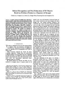
Two different views of 3-D mean vectors estimated from 2-D views of object Q2.

The training images include features only which belong to the object or which are caused by segmentation errors. The training of model densities for 3-D objects is done using 400 random views of each object. Again, all training images include a single object. Model generation is supervised with respect to the object class appearing in each image. The success of training algorithms using the EM algorithm depends crucially on an appropriate initialization of model parameters. Both the number n κ of model features and the parameters Bκ have to be set. The number of model features for each object class, which defines the structure of the model density, is assumed to be known in advance. This number n κ is defined by using the polyhedral object and counting the corners. Since normally distributed point features are assumed, mean vectors and covariance matrices are estimated during the training stage. In case of 2-D objects, 2-D mean vectors can be initialized using a single 2-D reference image. The initialization of 3-D model densities is based on lower-dimensional 2-D observations. For that reason, we start with mean vectors where the range component is set to zero. The model densities are estimated for point as well as for line features using the formulas described in Section 5. On average, in our experiments 5 EM iterations turn out to be sufficient for parameter estimation of 2-D models. The training of 3-D model densities is based on 2-D projections, and therefore besides the assignment

function the range data are missing. This slows down the convergence rate of EM iterations, however, we observed that in no example more than 15 EM iterations were required. The correctness of the estimation procedures of 3-D objects from 2-D views can be visualized by the estimated 3-D mean vectors of vertices. Figure 8 shows the estimated means for two different views of object Q2. We have to keep in mind that the mean vectors do not represent the reconstructed 3-D corners of the original object. The estimated 3-D mean vectors are probabilistic measurements computed from 2-D projections. The numerical analysis of errors is especially interesting in case of mean vectors. These parameters allow a concrete geometric interpretation. They represent the average coordinates of the model points. However, this is a probabilistic parameter which is influenced by segmentation errors, inaccuracies in camera calibration, quantization errors, etc. Table 1 summarized the Table 1.

Errors in 3-D mean estimates.

Object

Q1

Q2

Q3

Q4

#Corners

10

12

8

8

Max. depth (mm)

16

21

9

19

Min. deviation (mm)

1

0

1

1

Max. deviation (mm)

7

5

6

9

Mean deviation (mm)

3

3

3

3

3-D Objects

minimum, maximum and average deviation of the estimated coordinates in millimeters. We get an average error of 3 mm. 7.3.

Localization

The localization of objects corresponds to a global optimization problem of a continuous function. For that reason, we compare different global optimization algorithms. A fair measure for the quality of certain optimization algorithms is the required number of function evaluations for the detection of the global maximum. We test the adaptive random search (V1) (Ermakov and Zhiglyavskij, 1983), the adaptive random search method combined with the downhill-simplex algorithm (V2) (Press et al., 1988), see Section 6), simulated annealing for continuous functions (V3) (Corana et al. 1987), multistart techniques (V4) (Timmer, 1984), the grid-simplex algorithm (V5) (Press et al., 1988), and the pure probabilistic search (V6) (Boender et al., 1982). The data of the test set include 20 2-D views of a synthetic 3-D object (homogeneous background) and the corresponding 2-D point features. All selected optimization methods have several degrees of freedom. We adapt the parameters of the algorithms such that all optimization techniques find the prior known global maximum of the model density given a selected synthetic view. The pose estimate is considered to be correct if the mean error of back projected point features is below 10−5 . The number of function evaluations and the run time of this experiment are summarized in Table 2. The search is done in the five-dimensional pose space because orthographic projection is assumed. Our comparison shows that method V2 is the best optimization algorithm concerning the function evaluation criterion. For further experiments, we used the model density of object class P1 and generated 100 random views. For Table 2. Average number of density evaluations and run time of different global optimization algorithms. Method V1

Evaluations 10 010

Run time (sec) 25

V2

8 560

21

V3

41 300

102

V4

585 000

1446

V5

1 820 000

4488

V6

10 000 000

24602

247

the 3-D object Q1 we use 400 images. The correctness of pose estimates is checked by comparing the estimated pose parameters using the extrinsic parameters of the camera as references. The experiments with adaptive random search methods have shown the following results in case of the 2-D object:

! mean error in estimated angle is 2.5◦ with a variance ! the estimated translation vector is more robust and of 0.34◦ .

shows a mean error of 0.6 pixels and a variance of 0.05.

Regarding the 3-D object we get the following results:

! the global maximum could be found in 87% of the ! the global optimization in three stages (see Section 6) images,

is twice as fast as the optimization in the fivedimensional parameter space, and ! in average 5400 evaluations of the 1-D density function and 260 evaluations of the 2-D density functions are required. Some examples for pose computations in the presence of background features using ML estimates are illustrated in Fig. 9 for 2-D objects and in Fig. 10 for 3-D objects. The background shows also objects which are not elements of the model database. In these examples the object classes are assumed to be known. If the object classes are not known, two stages are required: pose estimation for all elements of the model database and subsequent classification. 7.4.

Classification

The pose estimation results show that within the classification experiments recognition rates for 3-D objects greater than 87% cannot be expected. Using pose dependent features, the correct localization is a necessary condition for classification. Errors are inherited from the pose estimation stage to the classification module. The class decision is based on the maximization of a posteriori probabilities p(!κ | O) (c.f. decision rule (1)). Herein, all objects are assumed to have identical prior probabilities. Table 3 shows the recognition rates for point and line features as well as the average runtime. Table 4 covers the same experiments for 3-D objects. The 2-D experiments consider 300 randomly chosen images of each class. The test set for 3-D objects contains 400 images of each class which were captured

248


Figure 9.

Figure 10.

Examples of scenes with heterogeneous background (left: gray-level image, middle: segmentation result, right: estimated pose).

Examples of scenes with heterogeneous background (left: gray-level image, middle: segmentation result, right: estimated pose).

by the robot’s camera. In all experiments learning and test set are disjoint. The recognition rate of 93% for the 2-D experiments seems satisfactory for the following reasons: the objects of classes P1 and P2 are symmetric with respect to the image plane and the probability to mix them up is a priori high. Object P4 has much less features than others. The size of P4 is similar to P1 and P2. If point or line features are used, a scene showing an element of object class P3 can be interpreted to show P4 and additional background features. These conclusions explain the lower recognition rates for P3 and P4, and also the restricted discriminating power of selected features. Another important observation is that the recognition rate does not increase with line features. This is due to the fact that the used segmentation algorithms decompose lines—characterized by initial and end points— into smaller parts. The splitting points have no geometric equivalent. Their appearance is randomly and the assumed normal distributions are not adequate in this case. This weakness of the statistical modeling of automatically segmented line features is also observed looking at 3-D examples. The recognition rate of about 70%

Table 3.

Run time and recognition rate of 2-D experiments. Recognition rate (%)

2-D object

Run time per image (sec)

Points

Lines

Points

Lines

P1

98

96

15

103

P2

94

94

17

111

P3

92

96

18

134

P4

90

85

10

77

Average

93

93

15

106

using point features decreases to 60% if line features are used for classification. Object class Q2 shows the best recognition rates. The L-shaped object differs from others in the height and the number of point features extremely. For that reason, point and line features show the highest discriminating power for this object. Object classes Q1 and Q3 represent slim objects. The image features corresponding to these objects are close to each other within the 2-D projections, and make the identification more difficult. This explains the low recognition rates of these objects.

3-D Objects

Table 4.

Run time and recognition rate of 3-D experiments. Recognition rate (%)

3-D object

Run time per image (sec)

Points

Lines

Points

Lines

Q1

47

44

154

660

Q2

78

82

161

692

Q3

58

36

154

638

Q4

89

76

155

501

Average

68

59

156

623

The discriminating power of geometric features will increase if 3-D instead of 2-D data were available for classification. The 2-D examples show that equal dimensions in model and image spaces allow recognition rates of more than 90%. 8.

Conclusions

Statistical methods become more and more popular in computer vision and they are of increasing interest. This paper has presented a novel and uniform approach to statistical modeling, localization, and classification of objects. We have discussed all the theoretical details as well as the implementation of a 2-D and 3-D object recognition system. Detailed tests were carried out. In general, the experimental results with a huge set of real images have proven the correctness and the practical use of proposed methods. The modeling of objects by non-geometric descriptions, but probabilistic density functions is remarkable: The application of the EM algorithm for automatic model generation leads to a powerful set of learning algorithms which overcome common problems associated with standard geometrical approaches. Marginalization and statistical independence, which are not available in geometrical settings, provide powerful tools to beat the curse of dimensionality, to reduce complexity, and to increase efficiency. The non-observable matching of image and model features is eliminated by marginalization. The independency of single assignments reduces the exponential complexity to a linear one. Furthermore, the pose space was decomposed by marginalization which results in a three stage pose estimation technique. The experiments concerning the involved global optimization problems have shown that also in the field of optimization theory, probabilistic algorithms are superior to deterministic methods. We presented reasonable probabilistic algorithms for pose estimation, where deterministic optimization was computationally prohibited.

249

Despite of the general mathematical framework and promising first experimental results, there still remain some general open problems: The pose computation corresponds to a parameter estimation problem, and is not based on geometrical constraints, like explicitly used feature correspondences and the analytical computation of pose parameters. Of course, an increase of the training data induces an increase of the reliability of estimated parameters. It seems natural that the use of multiple views will improve the pose estimation and object recognition rates; the more data, the more reliable estimates can be computed. Regarding the use of multiple views, the question is obvious, how to compute the most discriminating object views. Intelligent methods for viewpoint planning are required. The suggested framework allows to make use of information theory like entropy maximization techniques (Schiele and Crowley, 1998). It is well-known that a classifier is as good as its features. The used point and line features seem not to have the discriminating power as expected from reliable classifiers. Perhaps this is partially due to deficiencies of the segmentation algorithms. In addition, the applied features here are computed by non-statistical methods. Thus, the probabilistic approach does not cover all levels of object recognition by stochastic methods. Our future work will concentrate on the development of statistical algorithms which directly use graylevel images for object recognition and localization avoiding prior segmentation (Niemann and Hornegger, 2000). Glossary φ x , φ y , φz ∇ η & N K κ, λ !κ Nκ &

O ol & ol m & m

Eulerian angles nabla-operator Lagrange multiplier index of training view number of training views number of pattern classes indices of pattern classes class κ number of model features belonging to !κ set of observed features of view & l-th image feature l-th image feature of view & number of observed features number of observed features of view &

250


set of model features of "κ l-th model feature l-th model feature of "κ number of model features of class "κ θκ transforms object from model to the image B model parameters ˆ B estimation of B ˆ(i) estimation of B in the i-th iteration B parameters characterizing the BH background parameter characterizing cκ,l aκ,l Σ covariance matrix µ mean vector N (c; µ, Σ) normal (Gaussian) p.d.f. dimension of image space Do Dm dimension model space R, t affine mapping projection of class "κ θκ ζ assignment function assignments to class "κ ζκ ζ random vector induced by ζ ν neighborhood relation neighborhood relation of ok ! and ok !! νk ! ,k !! & ν banary random matrix of &-th view g dependency order index of model feature assigned to lk the k-th image feature Cκ cl cκ,l nκ

Acknowledgments The authors gratefully acknowledge the inspiring and concise remarks of the anonymous reviewers. This work was supported by Deutche Forschungsgemein schaft (DFG), grant SFB 603, TP BZ. Note 1. STACCATO: STAtistical ClAssification of Three-dimensional Objects.

References Altmann, S.L. 1986. Rotations, Quaternions, and Double Groups. Oxford University Press: Oxford. Anderson, T.W. 1958. An Introduction to Multivariate Statistical Analysis. John Wiley & Sons, Inc.: New York. Wiley Publications in Statistics. Bishop, C.M. 1995. Neural Networks for Pattern Recognition. Clarendon Press: Oxford.

Boender, C.G.E., Rinnoy Kan, A.H.G., Timmer, G.T., and Stougie, L. 1982. A stochastic method for global optimization. Mathematical Programming, 22:125–140. Cagliotti, V. 1994. Uncertainty minimization in the localization of polyhedral objects. IEEE Transactions on Pattern Analysis and Machine Intelligence (PAMI), 16(5):524–530. Corana, A., Marchesi, M., and Ridella, S. 1987. Minimizing multimodal functions of continuous variables with the “simulated annealing” algorithm. ACM Transactions on Mathematical Software, 13(3):209–217. Dubuisson, B. and Masson, M. 1993. A statistical decision rule with incomplete knowledge about classes. Pattern Recognition, 26(1):155–165. Ermakov, S.M. and Zhiglyavskij, A.A. 1983. On random search of global extremum. Probability Theory and Applications, 28(1):129–136. Faugeras, O. 1993. Three-Dimensional Computer Vision–A Geometric Viewpoint. MIT Press: Cambridge, Massachusetts. Fukunaga, K. 1990. Introduction to Statistical Pattern Recognition. Academic Press: Boston. Horn, B.K.P. 1986. Robot Vision. McGraw-Hill: New York. Hornegger, J. 1996. Statistical Modeling, Classification, and Localization of Objects (in German). Shaker Verlag: Aachen, Germany. Hornegger, J. 1997. Statistical modeling of relations for 3-D object recognition. In Proceedings of the International Conference on Acoustics, Speech, and Signal Processing (ICASSP), Munich, April 1997, vol. 4, IEEE Computer Society Press: Silver Spring, MD, pp. 3173–3176. Hornegger, J. and Niemann, H. 1994. A Bayesian approach to learn and classify 3-D objects from intensity images. In Proceedings of the 12th International Conference on Pattern Recognition (ICPR), Jerusalem, October 1994, IEEE Computer Society Press: Silver Spring, MD, pp. 557–559. Hornegger, J., Paulus, D., and Niemann, H. 1999. Probabilistic modeling in computer vision. In Handbook of Computer Vision and Applications, vol. 2, Jähne, B., Haussecker, H., and Geissler, P. Eds. Academic Press: London. Huang, X.D., Ariki, Y., and Jack, M.A. 1990. Hidden Markov Models for Speech Recognition. Edinburgh University Press: Edinburgh. Information Technology Series, Number 7. Jain, A.K. and Flynn, P.J. Eds. 1993. Three-Dimensional Object Recognition Systems. Amsterdam: Elsevier. Jelinek, F. 1998. Statistical Methods for Speech Recognition. MIT Press, Cambridge: Massachusetts. Kanatani, K. 1993. Geometric Computation for Machine Vision. Clarendon Press: Oxford. Oxford Engineering Science Series, Number 37. Kanatani, K. 1996. Statistical Optimization for Geometric Computation: Theory and Practice, vol. 18. Machine Intelligence and Pattern Recognition. Elsevier: Amsterdam. Kittler, J., Christmas, W.J., and Petrou, M. 1993. Probabilistic relaxation for matching problems in computer vision. In Proceedings of the 4th International Conference on Computer Vision (ICCV), Berlin, May 1993. IEEE Computer Society Press: Silver Spring, MD, pp. 666–673. Lawley, D.N. and Maxwell, A.E. 1971. Factor Analysis as a Statistical Method, 2nd edition. Butterworth & Co: London. Li, X., Parizeau, M., and Plamondon, R. 2000. Training hidden markov models with multiple observations: A combinatorial

3-D Objects

method. IEEE Transactions on Pattern Analysis and Machine Intelligence (PAMI), 22(4):371–377. McLachlan, G.J. and Krishnan, T. 1996. The EM Algorithm and Extensions. John Wiley & Sons, Inc.: New York. Wiley Series in Probability and Statistics. Mockus, J. 1989. Bayesian Approach to Global Optimization: Theory and Applications. Kluwer Academic Publishers: Dordrecht, Mathematics and Its Applications (Soviet Series). Murase, H. and Nayar, S.K. 1995. Visual learning and recognition of 3-D objects from appearance. International Journal of Computer Vision, 14(1):5–24. Niemann, H. and Hornegger, J. 2000. A novel probabilistic model for object recognition and pose estimation. International Journal of Pattern Recognition and Artificial Intelligence, accepted for publication. Paulus, D. and Hornegger, J. 1998. Applied pattern recognition: A practical introduction to image and speech processing in C++ 2nd edition. Vieweg: Braunschweig. Advanced Studies in Computer Science. Ponce, J., Zisserman, and Hebert, M. (Eds.) 1996. Object Representation in Computer Vision, volume 1144 of Lecture Notes in Computer Science. Springer: Heidelberg. Pope, A. 1995 Learning to recognize objects in images: Acquiring and using probabilistic models of appearance. Ph.D. Thesis, University of British Columbia, Vancouver. Press, W.H., Flannery, B.P., Teukolsky, S., and Vetterling, W.T. 1988. Numerical Recipes—the Art of Numerical Computing, C Version. Cambridge University Press: Cambridge.

251

Ripley, B.D. 1996. Pattern Recognition and Neural Networks. Cambridge University Press: Cambridge. Schiele, B. 1997. Object recognition using multidimensional receptive field histograms (English translation). Ph.D. Thesis, Institut National Polytechnique de Grenoble, Grenoble Cedex. Schiele, B. and Crowley, J.L. 1998. Transinformation for active object recognition. In Proceedings of the 6th International Conference on Computer Vision (ICCV), Bombay, january 1998: IEEE Computer Society Press: Silver Spring, MD, pp. 249–254. Timmer, G.T. 1984. Global optimization: A stochastic approach. Ph.D. Thesis, Erasmus University, Rotterdam. Trucco, E. and Verri, A. 1998. Introductory Techniques for 3-D Computer Vision. Prentice Hall: New York. Ullman, S. 1996. High-Level Vision: Object Recognition and Visual Cognition. MIT Press: Cambridge, MA. Wells, W.M., III, 1993. Statistical object recognition. Ph.D. Thesis, MIT, Department of Electrical Engineering and Computer Science, Cambridge, Massachusetts. Wells, W.M., III, 1997. Statistical approaches to feature-based object recognition. International Journal of Computer Vision, 21(2): 63–98. Winkler, G. 1995. Image Analysis, Random Fields and Dynamic Monte Carlo Methods, vol. 27. Applications of Mathematics. Springer: Heidelberg. Zhu, S.Z., Wu, Y., and Mumford, D. 1998. Filters, random fields and maximum entropy (frame): Towards a unified theory for texture modeling. International Journal of Computer Vision, 27(2): 127–159.

Probabilistic Modeling and Recognition of 3-D Objects - Pattern ...

Probabilistic Modeling and Recognition of 3-D Objects - Pattern ...

Suggest Documents

Pattern Recognition of 3D CAD Objects - CiteSeerX

Learning, Tracking and Recognition of 3D Objects

A Probabilistic Theory of Pattern Recognition

A Probabilistic Theory of Pattern Recognition

A Probabilistic Theory of Pattern Recognition

A Probabilistic Theory of Pattern Recognition

3D Objects Coding and Recognition Using Surface

Probabilistic 3D Object Recognition 1 Introduction - CiteSeerX

Probabilistic 3D Object Recognition 1 Introduction - CiteSeerX

Robust Recognition and Pose Estimation of 3D Objects Based on ...

3D Recognition and Segmentation of Objects in Cluttered ... - CiteSeerX

Pattern Recognition and Tracking Dynamic Objects with LIDAR

Keyframe-based Modeling and Tracking of Multiple 3D Objects

3d modeling of heritage objects by fringe projection and laser ...

Data Acquisition and Modeling of 3D Deformable Objects using

Keyframe-based Modeling and Tracking of Multiple 3D Objects

Segmentation and superquadric modeling of 3D objects - CiteSeerX

Morphological Modeling and Deformation of 3D Objects - Dynamic ...

Spatial Pattern Templates for Recognition of Objects with Regular

CAD-Based Recognition of 3D Objects in Monocular Images

3D Objects

active perception system for recognition of 3d objects in ... - CiteSeerX

Motion Pattern Analysis for Modeling and Recognition of Complex ...

3D Face Mesh Modeling for 3D Face Recognition - Semantic Scholar