Well-Definedness and Efficient Inference for Probabilistic Logic

arXiv:1110.0631v1 [cs.AI] 4 Oct 2011

Under consideration for publication in Theory and Practice of Logic Programming

1

Well-Definedness and Efficient Inference for Probabilistic Logic Programming under the Distribution Semantics FABRIZIO RIGUZZI ENDIF – University of Ferrara Via Saragat 1, I-44122, Ferrara, Italy E-mail: [email protected]

TERRANCE SWIFT CENTRIA – Universidade Nova de Lisboa E-mail: [email protected] submitted 22 November 2010; revised 15 April 2011; accepted 14 June 2011

Note: This article will appear in Theory and Practice of Logic Programming, c

Cambridge University Press, Abstract The distribution semantics is one of the most prominent approaches for the combination of logic programming and probability theory. Many languages follow this semantics, such as Independent Choice Logic, PRISM, pD, Logic Programs with Annotated Disjunctions (LPADs) and ProbLog. When a program contains functions symbols, the distribution semantics is well-defined only if the set of explanations for a query is finite and so is each explanation. Welldefinedness is usually either explicitly imposed or is achieved by severely limiting the class of allowed programs. In this paper we identify a larger class of programs for which the semantics is well-defined together with an efficient procedure for computing the probability of queries. Since LPADs offer the most general syntax, we present our results for them, but our results are applicable to all languages under the distribution semantics. We present the algorithm “Probabilistic Inference with Tabling and Answer subsumption” (PITA) that computes the probability of queries by transforming a probabilistic program into a normal program and then applying SLG resolution with answer subsumption. PITA has been implemented in XSB and tested on six domains: two with function symbols and four without. The execution times are compared with those of ProbLog, cplint and CVE. PITA was almost always able to solve larger problems in a shorter time, on domains with and without function symbols. KEYWORDS: Probabilistic Logic Programming, Tabling, Answer Subsumption, Logic Programs with Annotated Disjunction, Program Transformation

2

F. Riguzzi and T. Swift 1 Introduction

Many real world domains can only be represented effectively if we are able to model uncertainty. Accordingly, there has been an increased interest in logic languages representing probabilistic information, stemming in part from their successful use in Machine Learning. In particular, languages that follow the distribution semantics (Sato 1995) have received much attention in the last few years. In these languages a theory defines a probability distribution over logic programs, which is extended to a joint distribution over programs and queries. The probability of a query is then obtained by marginalizing out the programs. Examples of languages that follow the distribution semantics are Independent Choice Logic (Poole 1997), PRISM (Sato and Kameya 1997), pD (Fuhr 2000), Logic Programs with Annotated Disjunctions (LPADs) (Vennekens et al. 2004) and ProbLog (De Raedt et al. 2007). All these languages have the same expressive power as a theory in one language can be translated into another (Vennekens and Verbaeten 2003; De Raedt et al. 2008). LPADs offer the most general syntax as the constructs of all the other languages can be directly encoded in LPADs. When programs contain functions symbols, the distribution semantics has to be defined in a slightly different way: as proposed in (Sato 1995) and (Poole 1997): the probability of a query is defined with reference to a covering set of explanations for the query. For the semantics to be well-defined, both the covering set and each explanation it contains must be finite. To ensure that the semantics is well-defined, (Poole 1997) requires programs to be acyclic, while (Sato and Kameya 1997) directly imposes the condition that queries must have a finite covering set of finite explanations. Since acyclicity is a strong requirement ruling out many interesting programs, in this paper we propose a looser requirement to ensure the well-definedness of the semantics. We introduce a definition of bounded term-size programs and queries, which are based on a characterization of the Well-Founded Semantics in terms of an iterated fixpoint (Przymusinski 1989). A bounded term-size program is such that in each iteration of the fixpoint the size of true atoms does not grow indefinitely. A bounded term-size query is such that the portion of the program relevant to the query is bounded term-size. We show that if a query is bounded term-size, then it has a finite set of finite explanations that are covering, so the semantics is well-defined. We also present the algorithm “Probabilistic Inference with Tabling and Answer subsumption” (PITA) that builds explanations for every subgoal encountered during a derivation of a query. The explanations are compactly represented using Binary Decision Diagrams (BDDs) that also allow an efficient computation of the probability. Specifically, PITA transforms the input LPAD into a normal logic program in which the subgoals have an extra argument storing a BDD that represents the explanations for its answers. As its name implies, PITA uses tabling to store explanations for a goal. Tabling has already been shown useful for probabilistic logic programming in (Kameya and Sato 2000; Riguzzi 2008; Kimmig et al. 2009; Mantadelis and Janssens 2010; Riguzzi and Swift 2011). However, PITA is novel in

Well-Definedness and Efficient Inference for Probabilistic Logic Prog.

3

its exploitation of a tabling feature called answer subsumption to combine explanations coming from different clauses. PITA draws inspiration from (De Raedt et al. 2007), which first proposed to use BDDs for computing the probability of queries for the ProbLog language, a minimalistic probabilistic extension of Prolog; and from (Riguzzi 2007) which applied BDDs to the more general LPAD syntax. Other approaches for reasoning on LPADs include (Riguzzi 2008), where SLG resolution is extended by repeatedly branching on disjunctive clauses, and the CVE system (Meert et al. 2009) which transforms LPADs into an equivalent Bayesian network and then performs inference on the network using the variable elimination algorithm. PITA was tested on a number of datasets, both with and without function symbols, in order to evaluate its efficiency. The execution times of PITA were compared with those of cplint (Riguzzi 2007), CVE (Meert et al. 2009) and ProbLog (Kimmig et al. 2011). PITA was able to solve successfully more complex queries than the other algorithms in most cases and it was also almost always faster both on datasets with and without function symbols. The paper is organized as follows. Section 2 illustrates the syntax and semantics of LPADs over finite universes. Section 3 discusses the semantics of LPADs with function symbols. Section 4 defines dynamic stratification for LPADs, provides conditions for the well-definedness of the LPAD semantics with function symbols, and discusses related work on termination of normal programs. Section 5 gives an introduction to BDDs. Section 6 briefly recalls tabling and answer subsumption. Section 7 presents PITA and Section 8 shows its correctness. Section 9 discusses related work. Section 10 describes the experiments and Section 11 discusses the results and presents directions for future works. 2 The Distribution Semantics for Function-free Programs In this section we illustrate the distribution semantics for function-free program using LPADs as the prototype of the languages following this semantics. A Logic Program with Annotated Disjunctions (Vennekens et al. 2004) consists of a finite set of annotated disjunctive clauses of the form H1 : α1 ∨ . . . ∨ Hn : αn ← L1 , . . . , Lm . In such a clause H1 , . . . Hn are logical atoms, B1 , . . . , Bm logical literals, and α1 , P . . . , αn real numbers in the interval [0, 1] such that nj=1 αj ≤ 1. The term H1 : α1 ∨ . . . ∨ Hn : αn is called the head and L1 , . . . , Lm is called the body. Note that if n = 1 and α1 = 1 a clause corresponds to a normal program clause, also called P a non-disjunctive clause. If nj=1 αj < 1, the head of the clause implicitly contains an extra atom null that does not appear in the body of any clause and whose Pn annotation is 1 − j=1 αj . For a clause C, we define head(C) as {(Hi : αi )|1 ≤ i ≤ Pn Pn n} if i=1 αi = 1; and as {(Hi : αi )|1 ≤ i ≤ n} ∪ {(null : 1 − i=1 αi )} otherwise. Moreover, we define body(C) as {Li |1 ≤ i ≤ m}, Hi (C) as Hi and αi (C) as αi . If the LPAD is ground, a clause represents a probabilistic choice between the non-disjunctive clauses obtained by selecting only one atom in the head. As usual,

4

F. Riguzzi and T. Swift

if the LPAD T is not ground, T is assigned a meaning by computing its grounding, ground(T ). By choosing a head atom for each ground clause of an LPAD we get a normal logic program called a world of the LPAD (an instance of the LPAD in (Vennekens et al. 2004)). A probability distribution is defined over the space of worlds by assuming independence between the choices made for each clause. More specifically, an atomic choice is a triple (C, θ, i) where C ∈ T , θ is a minimal substitution that grounds C and i ∈ {1, . . . , |head(C)|}. (C, θ, i) means that, for the ground clause Cθ, the head Hi (C) was chosen. A set of atomic choices κ is consistent if (C, θ, i) ∈ κ, (C, θ, j) ∈ κ ⇒ i = j, i.e., only one head is selected for a ground clause. A composite choice κ is a consistent set of atomic choices. The probability P (κ) of a composite choice κ is the product of the probabilities of the Q individual atomic choices, i.e. P (κ) = (C,θ,i)∈κ αi (C). A selection σ is a composite choice that, for each clause Cθ in ground(T ), contains an atomic choice (C, θ, i) in σ. Since T does not contain function symbols, ground(T ) is finite and so is each σ. We denote the set of all selections σ of a program T by ST . A selection σ identifies a normal logic program wσ , called a world of T , defined as: wσ = {(Hi (C)θ ← body(C))θ|(C, θ, i) ∈ σ}. WT denotes the set of all the worlds of T . Since selections are composite choices, we can assign a probability Q to worlds: P (wσ ) = P (σ) = (C,θ,i)∈σ αi (C). Throughout this paper, we consider only sound LPADs, in which every world has a total model according to the Well-Founded Semantics (WFS) (Van Gelder et al. 1991). In this way, uncertainty is modeled only by means of the disjunctions in the head and not by the semantics of negation. Thus in the following, wσ |= A means that the ground atom A is true in the well-founded model of the program wσ 1 . In order to define the probability of an atom A being true in an LPAD T , note that the probability distribution over possible worlds induces a probability distribution over Herbrand interpretations by assuming P (I|w) = 1 if I is the well-founded model of w (I = W F M (w)) and 0 otherwise. We can thus compute the probability of an interpretation I as X X X P (w). P (I) = P (I, w) = P (I|w)P (w) = w∈WT

w∈WT

w∈WT ,I=W F M(w)

We can extend the probability distribution on interpretation to ground atoms by assuming P (aj |I) = 1 if Aj belongs to I and 0 otherwise, where Aj is a ground atom of the Herbrand base HT and aj stands for Aj = true. Thus the probability of a ground atom Aj being true, according to an LPAD T can be obtained as X X X P (aj ) = P (aj , I) = P (aj |I)P (I) = P (I). I

I

I⊆HT ,Aj ∈I

Alternatively, we can extend the probability distribution on programs to ground atoms by assuming P (aj |w) = 1 if Aj is true in w and 0 otherwise. Thus the 1

We sometimes abuse notation slightly by saying that an atom A is true in a world w to indicate that A is true in the (unique) well-founded model of w.

Well-Definedness and Efficient Inference for Probabilistic Logic Prog. probability of Aj being true is X X P (aj |w)P (w) = P (aj , w) = P (aj ) = w∈WT

w∈WT

X

5

P (w).

w∈WT ,w|=Aj

The probability of Aj being false is defined similarly. Example 1 Consider the dependency of sneezing on having the flu or hay fever: C1 C2 C3 C4

= = = =

strong sneezing(X) : 0.3 ∨ moderate sneezing(X) : 0.5 strong sneezing(X) : 0.2 ∨ moderate sneezing(X) : 0.6 f lu(david). hay f ever(david).

← ←

f lu(X). hay f ever(X).

This program models the fact that sneezing can be caused by flu or hay fever. The query moderate sneezing(david) is true in 5 of the 9 worlds of the program and its probability of being true is PT (moderate sneezing(david)) = 0.5·0.2+0.5·0.6+0.5·0.2+0.3·0.6+0.2·0.6 = 0.8 Even if we assumed independence between the choices for individual ground clauses, this does not represents a restriction, in the sense that this still allows to represent all the joint distributions of atoms of the Herbrand base that are representable with a Bayesian network over those variables. Details of the proof are omitted for lack of space.

3 The Distribution Semantics for Programs with Function Symbols If a non-ground LPAD T contains function symbols, then the semantics given in the previous section is not well-defined. In this case, each world wσ is the result of an infinite number of choices and the probability P (wσ ) is 0 since it is given by the product of an infinite number of factors all smaller than 1. Thus, the probability of a formula is 0 as well, since it is a sum of terms all equal to 0. The distribution semantics with function symbols was defined in (Sato 1995) and (Poole 2000). Here we follow the approach of (Poole 2000). A composite choice κ identifies a set of worlds ωκ that contains all the worlds associated to a selection that is a superset of κ: i.e., ωκ = {wσ |σ ∈ ST , σ ⊇ κ} We S define the set of worlds identified by a set of composite choices K as ωK = κ∈K ωκ Given a ground atom A, we define the notion of explanation, covering set of composite choices and mutually incompatible set of explanations. A composite choice κ is an explanation for A if A is true in every world of ωκ . In Example 1, the composite choice {(C1 , {X/david}, 1)} is an explanation for strong sneezing(david). A set of composite choices K is covering with respect to A if every world wσ in which A is true is such that wσ ∈ ωK . In Example 1, the set of composite choices K1 = {{(C1 , {X/david}, 2)}, {(C2, {X/david}, 2)}}

(1)

is covering for moderate sneezing(david). Two composite choices κ1 and κ2 are incompatible if their union is inconsistent, i.e., if there exists a clause C and a substitution θ grounding C such that (C, θ, j) ∈ κ1 , (C, θ, k) ∈ κ2 and j 6= k. A

6

F. Riguzzi and T. Swift

set K of composite choices is mutually incompatible if for all κ1 ∈ K, κ2 ∈ K, κ1 6= κ2 ⇒ κ1 and κ2 are incompatible. As illustration, the set of composite choices K2

=

{{(C1 , {X/david}, 2), (C2 , {X/david}, 1)}, {(C1 , {X/david}, 2), (C2, {X/david}, 3)},

(2)

{(C2 , {X/david}, 2)}} is mutually incompatible for the theory of Example 1. (Poole 2000) proved the following results • Given a finite set K of finite composite choices, there exists a finite set K ′ of mutually incompatible finite composite choices such that ωK = ωK ′ . • If K1 and K2 are both mutually incompatible finite sets of finite composite P P choices such that ωK1 = ωK2 then κ∈K1 P (κ) = κ∈K2 P (κ) Thus, we can define a unique probability measure µ : ΩT → [0, 1] where ΩT is defined as the set of sets of worlds identified by finite sets of finite composite choices: ΩT = {ωK |K is a finite set of finite composite choices}. It is easy to see that ΩT P is an algebra over WT . Then µ is defined by µ(ωK ) = κ∈K ′ P (κ) where K ′ is a finite mutually incompatible set of finite composite choices such that ωK = ωK ′ . As is the case for ICL, hWT , ΩT , µi is a probability space (Kolmogorov 1950). Definition 1 The probability of a ground atom A is given by P (A) = µ({w|w ∈ WT ∧ w |= A} If A has a finite set K of finite explanations such that K is covering then {w|w ∈ WT ∧ w |= A} = ωK and µ({w|w ∈ WT ∧ w |= A} = µ(ωK ) so P (A) is well-defined. In the case of Example 1, K2 shown in equation 2 is a finite covering set of finite explanations for moderate sneezing(david) that is mutually incompatible, so P (moderate sneezing(david)) = 0.5 · 0.2 + 0.5 · 0.2 + 0.6 = 0.8. 4 Dynamic Stratification of LPADs One of the most important formulations of stratification is that of dynamic stratification. (Przymusinski 1989) shows that a program has a 2-valued well-founded model iff it is dynamically stratified, so that it is the weakest notion of stratification that is consistent with the WFS. As presented in (Przymusinski 1989), dynamic stratification computes strata via operators on 3-valued interpretations – pairs of the form hT r; F ai, where T r and F a are subsets of the Herbrand base HP of a normal program P . Definition 2 For a normal program P , sets T r and F a of ground atoms, and a 3-valued interpretation I we define T rueP I (T r) = {A|A is not true in I; and there is a clause B ← L1 , ..., Ln in P , a ground substitution θ such that A = Bθ and for every 1 ≤ i ≤ n either Li θ is true in I, or Li θ ∈ T r};

Well-Definedness and Efficient Inference for Probabilistic Logic Prog.

7

F alseP I (F a) = {A|A is not false in I; and for every clause B ← L1 , ..., Ln in P and ground substitution θ such that A = Bθ there is some i (1 ≤ i ≤ n) such that Li θ is false in I or Li θ ∈ F a}. P (Przymusinski 1989) shows that T rueP I and F alseI are both monotonic, and deP P fines TI as the least fixed point of T rueI (∅) and FIP as the greatest fixed point of 2 F alseP I (HP ) . In words, the operator TI extends the interpretation I to add the new atomic facts that can be derived from P knowing I; FI adds the new negations of atomic facts that can be shown false in P by knowing I (via the uncovering of unfounded sets). An iterated fixed point operator builds up dynamic strata by constructing successive partial interpretations as follows.

Definition 3 (Iterated Fixed Point and Dynamic Strata) For a normal program P let W F M0 W F Mα+1 W F Mα

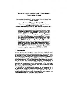
= h∅; ∅i; = W F Mα ∪ hTW F Mα ; FW F Mα i; S = β=0, s(T1,F), \+ s(T1,3). For this experiment, we query the probability of the HMM being in state 1 at time N for increasing values of N, i.e., we query the probability of s(N,1). In PITA and ProbLog, we did not use reordering of BDDs variables11 . In PITA we tabled on/2 and in ProbLog we tabled the same predicate using the technique described in (Mantadelis and Janssens 2010). The execution times of PITA, ProbLog, CVE and cplint are shown in Figure 2. In this problem tabling provides an impressive speedup, since computations can be reused often. 10 11

All experiments were performed on Linux machines with an Intel Core 2 Duo E6550 (2333 MHz) processor and 4 GB of RAM. For each experiment with PITA and ProbLog, we used either group sift automatic reordering or no reordering of BDDs variables depending on which gave the best results.

20

F. Riguzzi and T. Swift 1

cplint CVE ProbLog PITA

Time (s)

0.8 0.6 0.4 0.2 0 0

20

40

60

80

100

N

Fig. 2. Hidden Markov model.

The biological network programs compute the probability of a path in a large graph in which the nodes encode biological entities and the links represents conceptual relations among them. Each program in this dataset contains a non-probabilistic definition of path plus a number of links represented by probabilistic facts. The programs have been sampled from a very large graph and contain 200, 400, . . ., 10000 edges. Sampling was repeated ten times, to obtain ten series of programs of increasing size. In each program we query the probability that the two genes HGNC 620 and HGNC 983 are related. We used two definitions of path. The first, from (Kimmig et al. 2011), performs loop checking explicitly by keeping the list of visited nodes: path(X, Y ) path(X, Y, V, [Y |V ]) path(X, Y, V 0, V 1) arc(X, Y ) arc(X, Y )

← path(X, Y, [X], Z). ← arc(X, Y ). ← arc(X, Z), append(V 0, S, V 1), \ + member(Z, V 0), path(Z, Y, [Z|V 0], V 1). ← edge(X, Y ). ← edge(Y, X).

(3)

The second exploits tabling for performing loop checking: path(X, X). path(X, Y, ) ← path(X, Z), arc(Z, Y ). arc(X, Y ) ← edge(X, Y ). arc(X, Y ) ← edge(Y, X).

(4)

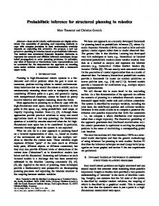
The possibility of using lists (that require function symbols) allowed in this case more modeling freedom. In PITA, the predicates path/2, edge/2 and arc/2 are tabled in both cases. For ProbLog we used its implementation of tabling for loop checking in the second program. As in PITA, path/2, edge/2 and arc/2 are tabled. We ran PITA, ProbLog and cplint on the graphs starting from the smallest program. In each series we stopped after one day or at the first graph for which the

Well-Definedness and Efficient Inference for Probabilistic Logic Prog. 10

PITA PITAt ProbLog ProbLogt cplint Time (s)

Answers

8 6 4 2 0

500

1000

1500 2000 Edges

2500

3000

(a) Number of successes.

10

6

10

4

10

2

10

0

10

−2

21

PITA PITAt ProbLog ProbLogt cplint

500

1000

1500 2000 Size

2500

3000

(b) Average execution times on the graphs on which all the algorithm succeeded.

Fig. 3. Biological graph experiments. 6

10

4

Time (s)

10

PITA PITAt ProbLog ProbLogt cplint

2

10

0

10

−2

10

500

1000

1500 2000 Size

2500

3000

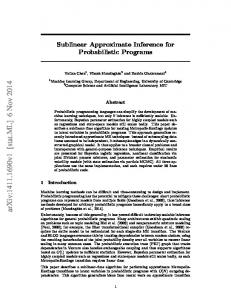
Fig. 4. Average exection times on the biological graph experiments. program ended for lack of memory12 . In cplint, PITA and ProbLog we used group sift reordering of BDDs variables. Figure 3(a) shows the number of subgraphs for which each algorithm was able to answer the query as a function of the size of the subgraphs, while Figure 3(b) shows the execution time averaged over all and only the subgraphs for which all the algorithms succeeded. Figure 4 alternately shows the execution times averaged, for each algorithm, over all the graphs on which the CVE was not applied to this dataset because the current version can not handle graph cycles.

10

6

10

6

10

4

10

10

2

10

0

10

−2

10

−4

4

0

20

40

60

PITA PITAdr ProbLog ProbLogdr cplint CVE 80 100

N

(a) bloodtype.

Fig. 5. Datasets from (Meert et al. 2009).

Time (s)

Time (s)

12

2

10

0

10

−2

10

−4

10

20

40

60 N

(b) growingbody.

PITA PITAdr ProbLog ProbLogdr cplint CVE 80 100

22

F. Riguzzi and T. Swift 6

4

Time (s)

10

2

10

PITA PITAdr ProbLog ProbLogdr cplint CVE

Time (s)

10

0

10

−2

10

−4

10

5

10 N

15

20

(a) growinghead.

10

6

10

4

10

2

10

0

10

−2

10

−4

PITA PITAdr ProbLog ProbLogdr cplint CVE

0

5

10

15

N

(b) uwcse.

Fig. 6. Datasets from (Meert et al. 2009).

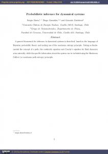
algorithm succeeded. In these Figures PITA and PITAt refers to PITA applied to path programs (3) and (4) respectively and similarly for ProbLog and ProbLogt. PITA applied to program (3) was able to solve more subgraphs and in a shorter time than cplint and all cases of ProbLog. On path definition (4), on the other hand, ProbLogt was able to solve a larger number of problems than PITAt and in a shorter time. For PITA the vast majority of time for larger graphs was spent on BDD maintenance. This shows that, even if tabling consumes more memory when finding the explanations, BDDs are built faster and use less memory, probably due to the fact that tabling allows less redundancy (only one BDD is stored for an answer) and supports a bottom-up construction of the BDDs, which is usually better. The four datasets of (Meert et al. 2009), served as a final suite of benchmarks. bloodtype encodes the genetic inheritance of blood type, growingbody contains programs with growing bodies, growinghead contains programs with growing heads and uwcse encodes a university domain. The best results for ProbLog were obtained by using ProbLog’s tabling in all experiments except growinghead. The execution times of cplint, ProbLog, CVE and PITA are shown in Figures 5(a) and 5(b), 6(a) and 6(b)13 . In the legend PITA means that dynamic BDD variable reordering was disabled, while PITAdr has group sift automatic reordering enabled. Similarly for ProbLog and ProbLogdr. In bloodtype, growingbody and growinghead PITA without variable reordering was the fastest, while in uwcse PITA with group sift automatic reordering was the fastest. These results show that variable reordering has a strong impact on performances: if the variable order that is obtained as a consequence of the sequence of BDD operations is already good, automatic reordering severely hinders performances. Fully understanding the effect of variable reordering on performances is subject of future work.

13

For the missing points at the beginning of the lines a time smaller than 10−6 was recorded. For the missing points at the end of the lines the algorithm exhausted the available memory.

Well-Definedness and Efficient Inference for Probabilistic Logic Prog.

23

11 Conclusion and Future Works This paper has made two main contributions. The first is the identification of bounded term-size programs and queries as conditions for the distribution semantics to be well-defined when LPADs contain function symbols. As shown in Section 4.2, bounded-term-size programs and queries sometimes include programs that other termination classes do not. Given the transformational equivalence of LPADs and other probabilistic logic programming formalisms that use the distribution semantics, these results may form a basis for determining well-definedness beyond LPADs. As a second contribution, the PITA transformation provides a practical reasoning algorithm that was directly used in the experiments of Section 10. The experiments substantiate the PITA approach. Accordingly, PITA should be easily portable to other tabling engines such as that of YAP, Ciao and B Prolog if they support answer subsumption over general semi-lattices. PITA is available in XSB Version 3.3 and later, downloadable from http://xsb.sourceforge.net. A user manual is included in XSB manual and can also be found at http://sites.unife.it/ml/pita. In the future, we plan to extend PITA to the whole class of sound LPADs by implementing the SLG delaying and simplification operations for answer subsumption; an implementation of tabling with term-depth abstraction (Section 6) is also underway. Finally, we are developing a version of PITA that is able to answer queries in an approximate way, similarly to (Kimmig et al. 2011). References Baselice, S., Bonatti, P., and Criscuolo, G. 2009. On finitely recursive programs. Theory and Practice of Logic Programming 9, 2, 213–238. Calimeri, F., Cozza, S., Ianni, G., and Leone, N. 2008. Computable functions in asp: Theory and implementation. In International Conference on Logic Programming. LNCS, vol. 5366. Springer, 407–424. Chen, W. and Warren, D. S. 1996. Tabled evaluation with delaying for general logic programs. Journal of the Association for Computing Machinery 43, 1, 20–74. De Raedt, L., Demoen, B., Fierens, D., Gutmann, B., Janssens, G., Kimmig, A., Landwehr, N., Mantadelis, T., Meert, W., Rocha, R., Santos Costa, V., Thon, I., and Vennekens, J. 2008. Towards digesting the alphabet-soup of statistical relational learning. In NIPS2008 Workshop on Probabilistic Programming, 13 December 2008, Whistler, Canada. De Raedt, L., Kimmig, A., and Toivonen, H. 2007. ProbLog: A probabilistic Prolog and its application in link discovery. In Internation Joint Conference on Artificial Intelligence. IJCAI, 2462–2467. Fuhr, N. 2000. Probabilistic datalog: Implementing logical information retrieval for advanced applications. Journal of the American Society of Information Sciences 51, 2, 95–110. Kameya, Y. and Sato, T. 2000. Efficient EM learning with tabulation for parameterized logic programs. In International Conference on Computational Logic. LNCS, vol. 1861. Springer, 269–284. Kimmig, A., Demoen, B., De Raedt, L., Costa, V. S., and Rocha, R. 2011. On the implementation of the probabilistic logic programming language problog. Theory and Practice of Logic Programming 11, Special Issue 2-3, 235–262.

24

F. Riguzzi and T. Swift

Kimmig, A., Gutmann, B., and Santos Costa, V. 2009. Trading memory for answers: Towards tabling ProbLog. In International Workshop on Statistical Relational Learning, 2-4 July 2009, Leuven, Belgium. KU Leuven. Kolmogorov, A. N. 1950. Foundations of the Theory of Probability. Chelsea Publishing Company. Mantadelis, T. and Janssens, G. 2010. Dedicated tabling for a probabilistic setting. In Technical Communications of the International Conference on Logic Programming. LIPIcs, vol. 7. Schloss Dagstuhl - Leibniz-Zentrum fuer Informatik, 124–133. Meert, W., Struyf, J., and Blockeel, H. 2009. CP-Logic theory inference with contextual variable elimination and comparison to BDD based inference methods. In International Conference on Inductive Logic Programming. LNCS, vol. 5989. Springer, 96–109. Muggleton, S. 2000. Learning stochastic logic programs. Electronic Transactions on Artificial Intelligence 4, B, 141–153. Poole, D. 1997. The independent choice logic for modelling multiple agents under uncertainty. Artificial Intelligence 94, 1-2, 7–56. Poole, D. 2000. Abducing through negation as failure: stable models within the independent choice logic. Journal of Logic Programming 44, 1-3, 5–35. Przymusinski, T. 1989. Every logic program has a natural stratification and an iterated least fixed point model. In Symposium on Principles of Database Systems. ACM Press, 11–21. Riguzzi, F. 2007. A top down interpreter for LPAD and CP-logic. In Congress of the Italian Association for Artificial Intelligence. LNAI, vol. 4733. Springer, 109–120. Riguzzi, F. 2008. Inference with logic programs with annotated disjunctions under the well founded semantics. In International Conference on Logic Programming. LNCS, vol. 5366. Springer, 667–771. Riguzzi, F. and Swift, T. 2011. The PITA system: Tabling and answer subsumption for reasoning under uncertainty. Theory and Practice of Logic Programming, International Conference on Logic Programming Special Issue 11, 4-5, 433–449. Sagonas, K., Swift, T., and Warren, D. S. 2000. The limits of fixed-order computation. Theoretical Computer Science 254, 1-2, 465–499. Sato, T. 1995. A statistical learning method for logic programs with distribution semantics. In International Conference on Logic Programming. MIT Press, 715–729. Sato, T. and Kameya, Y. 1997. Prism: A language for symbolic-statistical modeling. In International Joint Conference on Artificial Intelligence. IJCAI, 1330–1339. Swift, T. 1999a. A new formulation of tabled resolution with delay. In Recent Advances in Artifiial Intelligence. LNAI, vol. 1695. Sringer, 163–177. Swift, T. 1999b. Tabling for non-monotonic programming. Annals of Mathematics and Artificial Intelligence 25, 3-4, 201–240. Tamaki, H. and Sato, T. 1986. OLDT resolution with tabulation. In International Conference on Logic Programming. LNCS, vol. 225. Springer, 84–98. Thayse, A., Davio, M., and Deschamps, J. P. 1978. Optimization of multivalued decision algorithms. In International Symposium on Multiple-Valued Logic. IEEE Computer Society Press, 171–178. van Gelder, A. 1989. The alternating fixpoint of logic programs with negation. In Symposium on Principles of Database Systems. ACM, 1–10. Van Gelder, A., Ross, K. A., and Schlipf, J. S. 1991. The well-founded semantics for general logic programs. Journal of the Association for Computing Machinery 38, 3, 620–650.

Well-Definedness and Efficient Inference for Probabilistic Logic Prog.

25

Vennekens, J. and Verbaeten, S. 2003. Logic programs with annotated disjunctions. Tech. Rep. CW386, K. U. Leuven. Vennekens, J., Verbaeten, S., and Bruynooghe, M. 2004. Logic programs with annotated disjunctions. In International Conference on Logic Programming. LNCS, vol. 3131. Springer, 195–209.

Appendix A Proof of Well-Definedness Theorems (Section 4.1) To prove Theorem 1 we start with a lemma that states one half of the equivalence, and also describes an implication of the bounded term-size property for computation. Lemma 2 Let P be a normal program with the bounded term-size property. Then 1. Any atom in W F M (P ) has a finite stratum, and was computed by a finite number of applications of T rueP . 2. There are a finite number of true atoms in W F M (P ). Proof For 2), note that bounding the size of θ as used in Definition 2 bounds the size of the ground clause B ← L1 , ..., Ln , and so bounds the size of T rueP I (T r) for any I, T r ⊆ HP . Since the true atoms in W F M (P ) are defined as a fixed-point of T rueP I for a given I, there must be a finite number of them. Similarly, since the size of θ is bounded by an integer L, and since T rueP I is mono(∅) reaches its fixed point in a finite number of applications, tonic for any I T rueP I and in fact only a finite number of applications of T rueP I are required to compute true atoms in W F M (P ). In addition, it can be the case that TIP 6= I only a finite number of times, so that W F M (P ) can contain only a finite number of strata. Theorem 1 Let P be a normal program. Then W F M (P ) has a finite number of true atoms iff P has the bounded term-size property. Proof The ⇐ implication was shown by the previous Lemma, so that it remains to prove that if W F M (P ) has a finite number of true atoms, then P has the bounded termsize property. To show this, since the number of true atoms in W F M (P ) is finite, all derivations of true atoms using T rueP I (T r) of Definition 2 can be constructed using only a finite set of ground clauses. For this to be possible, the maximum term size of any literal in any such clause is finitely bounded, so that P has the bounded term-size property. Theorem 2 Let T be a sound bounded term-size LPAD, and let A ∈ HT . Then A has a finite set of finite explanations that is covering.

26

F. Riguzzi and T. Swift

Proof Let T be an LPAD and w be a world of T . Each clause Cground in w is associated with a choice (C, θ, i), for which C and i can both be taken as finite integers. We term (C, θ, i) the generators of Cground . By Theorem 1 each world w of T has a finite number of true atoms, and a maximum size Lw of any atom in such a world. We prove that the maximum LT of all such worlds has a finite upper bound. We first consider the case in which T does not contain negation. Consider a world w whose well-founded model has the finite bound Lw on the size of the largest atoms. We show that Lw can not be arbitrarily large. Since Lw is finite, all facts in T must be ground and all clauses range-restricted: otherwise some possible world of T would contain an infinite number of true atoms and so would not be bounded term-size by Theorem 1. There must be some set G of generators which acts on a chain of interpretations I0 ⊂ I1 ⊂ In ⊂ W F M (w), where I0 is some superset of the facts in w, and the maximum size of any atom in Ii is strictly increasing. Because W F M (w) is finite and T is definite, the set of generators G must be finite. We first show that G must contain generators (C ′ , θ, i) and (C ′ , θ′ , j) for at least one disjunctive clause C ′ . If not, then either 1) Lw would be infinite as there would be some recursion in which term size increases indefinitely; or 2) if there is no such recursion that indefinitely increases the size of terms and no disjunctive clauses, Lw could not be arbitrarily large and this would prove the property. In fact, without disjunction the set of clauses causing the recursion would produce an infinite model. With disjunction, eventually a different head is chosen and the recursion is stopped. Consider then, for some set D of disjunctive clauses, the set Dexpand of generators must be used to derive (perhaps indirectly) atoms whose size is strictly greater than the maximal size of an atom in In , while another set of generators Dstop must be used to stop the production of larger atoms, since W F M (w) is finite. However, if such a situation were the case, there must also be a world winf in which for ground clauses for D whose grounding substitution is over a certain size, only the set Dexpand of generators is chosen and Dstop is never chosen. The well-founded model for winf would then be infinite, against the hypothesis that T is bounded term-size. The preceding argument has shown that since there is an overall bound on the size of the largest atom in any world for T , T has a finite number of different models, each of which is finite. As each model is finite, there is a finite number of ground clauses that determine each model by deriving the positive atoms in the model. Each such clause is associated with an atomic choice, and the set of these clauses corresponds to a finite composite choice. The set of these composite choices corresponding to models in which the query A is true represent a finite set of finite explanations that is covering for A. Although the preceding paragraph assumed that T did not contain negation, the assumption was made only for simplicity, so that details of strata need not be considered. The argument for normal programs is essentially the same, constituting an induction where the above argument is made for each stratum. Because Definition 2 specifies that an atom can be added to an interpretation only once, there can only

Well-Definedness and Efficient Inference for Probabilistic Logic Prog.

27

be a finite number of strata in which some true atom is added, so that there will be only a finite number of strata overall. Since there are only a finite number of strata, each of which has a finite number of applications of T rueP I (T r), a finite bound L can be constructed so that T fulfills the definition of bounded term-size. Appendix B Proof of the Termination Theorem for Tabling (Section 6) Theorem 3 Let P be fixed-order dynamically stratified normal program, and Q a bounded term-size query to P . Then there is an SLG evaluation of Q to P using term-depth abstraction that finitely terminates. Proof SLG has been proven to terminate for other notions of bounded term-size queries, so here we only sketch the termination proof. First, we note that (Sagonas et al. 2000) guarantees that if P is a fixed-order stratified program, then there is an an SLG evaluation E of P that does not require the use of the SLG Delaying, Simplification or Answer Completion operations, and by implication no forest of E contains a conditional answer. Such an evaluation is termed delay-minimal. Note that Definition 4 constrains only the bindings used in T rueP I , and these constraints may not apply ground atoms that are undefined in the W F M (P ). As a result, condition answers, if they are not simplified or removed by Simplification or Answer Completion may not have a bounded term-size. This situation is avoided by delay-minimal evaluations. Next, we assume that all negative selected literals are ground. This assumption causes no loss of generality as the evaluation will flounder and so terminate finitely if a non-ground negative literal is selected. Given this context, the proof uses the forest-of-trees model (Swift 1999a) of SLG (Chen and Warren 1996). • We consider as an induction basis the case when Q is in stratum 0 – that is, when Q can be derived without clauses that contain negative literals, or is part of an unfounded set S of atoms and clauses for atoms in S do not contain negative literals. As argued in Section 6, the use of term-depth abstraction ensures that an SLG evaluation E of a query Q to a program with bounded term-size has only a finite number of trees. In addition, since SLG works on the original clauses of a program P and P is finite, (although ground(P ) may not be), there can be only a finite number of clauses resolvable against the root of any tree via Program Clause Resolution, and so the root of each SLG tree can contain only a finite number of children. Finally, to show that each interior node has a finite number of children, we consider that there can only be a finite number of answers to any subgoal upon which Q depends. This follows from the fact that E is delay-minimal and so produces no conditional answers, together with the the bound of Definition 4 that ensures a program is bounded term-size. As a result, there are only a finite number of nodes that are produced through Answer Return. These observations together ensure that each tree in any SLG forest of E is finite. Since each operation (including the SLG Completion operation, which does not add nodes to a forest) is applicable

28

F. Riguzzi and T. Swift

only one time to a given node or set of nodes in an evaluation (i.e. executing an SLG operation removes the conditions for its applicability) the evaluation E itself must be finite and statement holds for the induction basis. • For the induction step, we assume the statement holds for queries whose (fixedorder) dynamic strata is less than N to show that the statement will hold for a query Q at stratum N as well. As indicated above, we use a delay-minimal SLG evaluation E that does not require Delaying, Simplification or Answer Completion operations. For the induction case, the various SLG operations that do not include negation will only produce a finite number of trees and a finite number of nodes in each tree as described in the induction basis. However if there is a node N in a forest with a selected negative literal ¬A, the SLG operation Negation Return is applicable. In this case, a single child will be produced for N and no further operations will be applicable to N . Thus any forest in E will have a finite number of finite trees, and since all operations can be applied once to each node, as before E will be finite, so that the statement holds by induction.

Appendix C Proof of the Correctness Theorems for PITA (Section 8) The next theorem addresses the correctness of the PITA evaluation. As discussed in Section 8, the BDDs of the PITA transformation are represented as ground terms, while BDD operations, such as and/3, or/3 etc. are infinite relations on such terms. The PITA transformation also uses the predicate get var n/4 whose definition in Section 7 is: get var n(R, S, P robs, V ar) ← (var(R, S, V ar) → true; length(P robs, L), add var(L, P robs, V ar), assert(var(R, S, V ar))). This definition uses a non-logical update of the program, and so without modifications, it is not suitable for our proofs below. Alternately, we assume that ground(T ) is augmented with a (potentially infinite) number of facts of the form var(R, [], V ar) for each ground rule R (note that no variable instantiation is needed in the second argument of var/3 if it is indexed on ground rule names). Clearly, the augmentation of T by such facts has the same meaning as get var n/4, but is simply done by an a priori program extension rather than during the computation as in the implementation. Lemma 1 Let T be an LPAD and Q a bounded term-size query to T . Then the query P IT AH (Q) to P IT A(T ) has bounded term-size. Proof Although TQ (Definition 6) has bounded term-size, we also need to ensure that P IT A(TQ ) has bounded term-size, given the addition of the BDD relations and/3, or/3, etc. along with the var/3 relations mentioned above. Both var/3 and the BDD relations are functional on their input arguments (i.e.

Well-Definedness and Efficient Inference for Probabilistic Logic Prog.

29

the first two arguments of var/3, and/3, or/3. etc. (cf. Section 7). Therefore, for T the body of a clause C that was true in an application of T rueI Q there are exactly P IT A(TQ ) n bodies that are true in an application of T rueI , where n is the number of heads of C. Thus the size of every ground substitutions in every iteration of P IT A(TQ ) T rueI is bounded as well. Note that since P IT A(T ) and P IT AH (Q) are both syntactic transformations, the theorem applies even if the LPAD isn’t sound. Theorem 4 Let T be a fixed-order dynamically stratified LPAD and Q a ground bounded term-size atomic query. Then there is an SLG evaluation E of P IT AH (Q) against P IT A(TQ ), such that answer subsumption is declared on P IT AH (Q) using BDDdisjunction where E finitely terminates with an answer Ans for P IT AH (Q) and BDD(Ans) represents a covering set of explanations for Q. Proof (Sketch) The proof uses the forest-of-trees model (Swift 1999a) of SLG (Chen and Warren 1996). Because T is fixed-order dynamically stratified, queries to T can be evaluated using SLG without the delaying, simplification or answer completion operations. Instead, as (Sagonas et al. 2000) shows, only the SLG operations new subgoal, program clause resolution, answer return and negative return are needed. Since T is fixed-order dynamically stratified, it is immediate from inspecting the transformations of Section 7 together with the fact that the BDD relations are functional that P IT A(T ) is also fixed-order dynamically stratified as is P IT A(T )Q . However, Theorem 3 must be extended to evaluations that include answer subsumption, which we capture with a new operation Answer Join to perform answer subsumption over an upper semi-lattice L. Without loss of generality we assume that a given predicate of arity m > 0 has had answer subsumption declared on its mth argument and we term the first m − 1 arguments non-subsuming arguments. We recall that a node N is an answer in an SLG tree T if N has no unresolved goals and is a leaf in T . Accordingly, creating a child of N with a special marker f ail is a method to effectively delete an answer (cf. (Swift 1999a)). • Answer Join: Let an SLG forest Fn contain an answer node N = Ans ← where the predicate for Ans has been declared to use answer subsumption over a lattice L for which the join operation is decidable, and let the arity of Ans be m > 0. Further, let A be the set of all answers in Fn that are in the same tree, TN , as N and for which the non-subsuming arguments are the same as Ans. Let Join be the L-join of all the final arguments of all answers in A. — If (Ans ←){arg(m, Ans)/Join} is not an answer in TN , add it as a child of N , and add the child f ail to all other answers in A. — Otherwise, if (Ans ←){arg(m, Ans)/Join} is answer in TN , create a child f ail for N .

30

F. Riguzzi and T. Swift

For the proof, the first item to note is that since TQ is bounded term-size, any clauses on which Q depends that give rise to true atoms in the well-founded model of any world of T must be be range-restricted – otherwise since T has function symbols, TQ would have an infinite model and not be bounded term-size. Given this, it is then straightforward to show that P IT A(T )Q is also range-restricted and that any answer A of P IT AH (Q) will be ground (cf. (Muggleton 2000)). Accordingly, the operation Answer Join will be applicable to any subgoal with a non-empty set of answers. We extend Theorem 3 and Lemma 1 to show that since P IT A(T )Q has the bounded term-size property, a SLG evaluation of a query P IT AH (Q) to P IT A(T )Q will terminate. Because the join operation for L is decidable, computation of the join will not affect termination properties. Let TN be a tree whose root subgoal is a predicate that uses answer subsumption. Then each time a new answer node N is added to TN there will be one new Answer Join operation that becomes applicable for N . Let A be a set of answers in TN as in the definition of Answer Join. Then applying the Answer Join operation will either 1) create a child of N that is a new answer and “delete” |A| answers by creating children for them of the form f ail; or 2) “delete” the answer N by creating a child f ail of N . Clearly any answer can be deleted at most once, and each application of the Answer Join operation will delete at least one answer in TN . Accordingly, if TN contains N um answers, there can be at most N um applications of Answer Join for answers in TN . Using these considerations it is straightforward to show that termination of bounded term-size programs holds for SLG evaluations extended with answer subsumption 14 . Thus, the bounded term-size property of P IT A(T )Q together with Theorem 2 imply that there will be a finite set of finite explanations for P IT AH (Q), and the preceding argument shows that SLG extended with Answer Join will terminate on the query P IT AH (Q). It remains to show that an answer Ans for P IT AH (Q) in the final state of E is such that BDD(Ans) represents a covering set of explanations for Q. That BDD(Ans) contains a covering set of explanations can be shown by induction on the number of BDD operations. For the induction basis it is easy to see that the operations zero/1 and one/1 are covering for false and true atoms respectively. • Consider an “and” operation in the body of a clause. For the inductive assumption, BBi−1 and Bi both represent finite set of explanations covering for L1 , . . . , Li−1 and Li respectively. Let Fi−1 , Fi′ , and Fi be the formulas expressed by BBi−1 , Bi , and BBi respectively. These formulas can be represented in disjunctive normal form, 14

As an aside, note that due to the fact that Answer Join deletes all answers in A except the join, it can be shown by induction that immediately after an Answer Join operation is applied to Ans in a tree TN , there will be only one “non-deleted” answer in TN with the same non-subsuming bindings as Ans. Accordingly, if the cost of computing the join is constant, the total cost of N um Answer Join operations will be N um. Based on this observation, the implementation of PITA can be thought of as applying an Answer Join operation immediately after a new answer is derived in order to avoid returning answers that are not optimal given the current state of the computation.

Well-Definedness and Efficient Inference for Probabilistic Logic Prog.

31

in which every disjunct represents an explanation. Fi is obtained by multiplying Fi−1 and Fi′ so, by algebraic manipulation, we can obtain a formula in disjunctive normal form in which every disjunct is the conjunction of two disjuncts, one from Fi−1 and one from Fi′ . Every disjunct is thus an explanation for the body prefix up to and including Li . Moreover, every disjunct for Fi is obtained by conjoining a disjunct for Fi−1 with a disjunct for Fi′ . • In the case of a “not” operation in the body of a clause, let Li be the negative literal ¬D. Then for BNi the BDD produced by D, not(BNi , Bi ) simply negates this BDD to produce a covering set of explanations for ¬D. • In the case of an “or” operation between two answers, the resulting BDD will represents the union of the set of explanations represented by the BDDs that are joined. Since the property holds both for the induction basis and the induction step, the set of explanations represented by BDD(Ans) is covering for the query.