http://irc.nrc-cnrc.gc.ca
Processing laser range image for the investigation on the long-term performance of ductile iron pipe NRCC-49697 Liu, Z.; Krys, D.; Rajani, B.; Najjaran, H.
A version of this document is published in / Une version de ce document se trouve dans: Nondestructive Testing and Evaluation, v. 23, no. 1, March 2008, pp. 65-75 doi: 10.1080/10589750701775858
The material in this document is covered by the provisions of the Copyright Act, by Canadian laws, policies, regulations and international agreements. Such provisions serve to identify the information source and, in specific instances, to prohibit reproduction of materials without written permission. For more information visit http://laws.justice.gc.ca/en/showtdm/cs/C-42 Les renseignements dans ce document sont protégés par la Loi sur le droit d'auteur, par les lois, les politiques et les règlements du Canada et des accords internationaux. Ces dispositions permettent d'identifier la source de l'information et, dans certains cas, d'interdire la copie de documents sans permission écrite. Pour obtenir de plus amples renseignements : http://lois.justice.gc.ca/fr/showtdm/cs/C-42
Processing Laser Range Image for the Investigation on the Long-Term Performance of Ductile Iron Pipe Zheng Liu, *
1*
, Dennis Krys*, Balvant Rajani*, and Homayoun Najjaran**
Institute for Research in Construction, National Research Council Canada, Montreal Road 1200, Ottawa, Ontario K1A 0R6 Canada ** School of Engineering (Okanagan Campus), University of British Columbia, Kelowna, British Columbia V1V 1V7 Canada
1 Corresponding
1366.
author: E-mail:
[email protected], Tel: (613)993-3806, Fax: (613)993-
Abstract Prediction of service life of ductile iron pipe is carried out using the information on pipe condition, backfill/soil properties, and corrosion rates, as well as historical failure records. Among the factors that affect pipe condition, external pitting corrosion is a prominent variable contributing to the disintegrity of the pipe. A pipe scanner equipped with a laser displacement sensor was used to measure pitting corrosion. The pipe scanner can generate an accurate topographic mapping of the outer surface of the pipe. In order to accelerate the scanning process, a scan with reduced resolution is preferred. An image of higher resolution can be obtained with interpolation methods afterwards. Different interpolation methods are compared in term of the accuracy. To establish the statistical model, we need to identify and characterize each corroded area from the scanned laser range images. Quantitative description of the corroded areas, such as size, percentage of material loss, and location, needs to be generated and kept in a database for modeling and prediction purpose. This paper describes the procedure to carry out the process of the laser scan of ductile iron pipe.
1
Introduction
Ductile iron (DI) became the pipe material of choice for many municipalities from the late 1960s. The oldest DI pipes are approaching fifty years of age. However, DI pipe condition is not determined by age only. Many other factors, such as the electrochemical and physical properties of surrounding soils, can have an impact on the pitting corrosion of the DI pipe, which is widely acknowledged as a factor governing the pipes’ long-term durability. This requires the development of a statistical model that can relate current condition of pipes and corrosion rates with existing soil properties [1]. A comprehensive review of the state-ofart of modeling techniques can be found in references [2, 3]. The mechanism of pit growth has not been fully explored and understood. The quantification of the temporal and spatial distribution of pitting corrosion as well as the pitting growth rate still remains a challenge for the study of predicting service life of DI mains. As part of a research project sponsored by American Water Works Association Research Foundation (AwwaRF) and National Research Council Canada (NRC) on long-term performance of ductile iron pipe, a field testing program was initiated to investigate the soil environment and determine the corrosion rates from selected locations and DI pipe segments. To quantify pitting corrosion, a DI pipe scanning system, which is based on a laser displacement sensor, was developed at the NRC Institute for Research in Construction (IRC). The scanning system can accurately map pitting corrosion with a high resolution laser range image. From the acquired image, the pitting corrosion can be further characterized with quantitative measurements like area, maximum pit depth, percentage of material loss, etc. The scanning of DI pipe with the laser displacement sensor can be used for two purposes, i.e. modeling and predicting. At the modeling stage, the laser scan data can be used to discern the relationship between pitting corrosion and pipe condition. Input variables to such a model may also include historical failure rates, soil properties, and any potential nondestructive inspection results. Once this relationship is determined; laser measurements from a small sample (portion) of the total pipe length can be used to assess the condition of 1
the whole pipe length at the predicting stage. In this paper, a procedure to process laser range image and to extract the information of pitting corrosion for ductile iron pipe is described. Each corroded area is identified in terms of the percentage of material loss. The information about the pitting corrosion such as area, percentage of material loss, maximum pit depth, and location can be stored in a database to help establish statistical models for estimating the residual life of ductile iron pipes. The rest of the paper is organized as follows. Section 2 introduces the laser scanning system for the ductile iron pipe. The procedure to process the laser range image is described in section 3. In this section, each processing step is explained in detail with a sample scanning image. The summary of this paper can be found in the final section 4.
2
The Laser Scanning System
The scanning system with a laser displacement sensor is shown in Figure 1. A displacement laser head is mounted on a linear scanner at a constant distance of 50 mm (see Figure 1(b)). The laser displacement sensor that the scanning system uses is a Sick OD50-10P840 manufactured by SICK company [4]. With its current settings, this laser displacement sensor has a range of 50 ± 10 mm and takes a measurement every millisecond at an accuracy of 30 µm [5]. This system is currently used as a research tool and could be a basis for developing in-service system. If the pipe is not mounted perfectly, then as the pipe rotates, the distance between the surface of the pipe and the laser range finder can change, which will show up as a rotated (tilted) pipe surface. Post processing, described in the next section, is applied to correct the tilt in an improperly mounted pipe because it is almost impossible to mount a pipe with the same accuracy as the laser displacement sensor. This allows the pipe scanner to return highly accurate measurements, even when the pipe is slightly tilted. The scanning system has the ability to accommodate DI pipes of diameter 150 ∼ 300 mm
2
(a) The whole scanning system.
(b) The laser head.
Figure 1: The picture of the laser scanning system for ductile iron pipe.
and maximum length of 1070 mm. The linear actuator moves the laser displacement sensor at a speed of 650 mm/s with a reproducible accuracy of 0.1 mm. This allows a 880 mm long (150 mm diameter) pipe to be scanned in less then 10 minutes at a resolution of 1.5 mm. The data acquisition software that controls the scanning system allows the user to choose between scanning the whole pipes surface or just a segment of it. The user needs to enter specific parameters such as desired scanning resolution and diameter of the pipe. The software will take these parameters and determine the details that are required to scan the pipe with the desired settings.
3 3.1
Processing Laser Range Image The Procedure
The procedure to process the laser range image is shown in Figure 2. The first step is the preprocessing and correction. The scanner is accelerated or deaccelerated at the beginning or the end of a scan by the linear actuator. This will result in scanned points nonuniformly distributed on a gird as illustrated in Figure 3. Although the laser displacement sensor is very precise, the mechanical system to operate the sensor is not, because the mechanical system cannot reach a comparable precision as the laser sensor. The pipe and linear actuator
3
cannot be perfectly mounted on a common axis. Therefore, a correction of the scanned data is needed.
Figure 2: The procedure to create a database from laser scanning.
Figure 3: The actual distribution of scanning points on a grid.
The second step is using interpolation method to generate a image of a higher resolution. A high-resolution laser scanning is a time-consuming process. A faster scan at a reasonable time is preferred either in the lab or in the field. However, low-resolution scan lose the details of surface roughness. Interpolation method can be applied to solve this problem. Pitting corrosion is first characterized by the pitting depth, which is identified by the percentage of material loss. A series of binary images are obtained by applying a set of threshold values representing different percentages of material loss. Each binary image is further characterized by labeling every region with corresponding information like area, maximum depth, location, etc. Such information can be stored in a database for modeling or 4
predicting use.
3.2
Preprocessing and Correction
The acquired raw data requires preprocessing as explained below. If a desired resolution of 1.5 mm is required, then the values read from the laser scan are not guaranteed to be spaced 1.5 mm apart. Instead it is only guaranteed to have at least one value for every 1.5 mm. The reason for this is that the laser is read at a continuous rate of 1 reading every millisecond. The linear actuator tries to maintain a constant velocity to achieve the desired spacing between readings. Because the linear actuator has a limited top speed and cannot achieve infinite acceleration, the grouping of the data points will always be closer then what is desired. For example at the ends of the track the linear actuator has to accelerate to the desired velocity and then decelerate to stop. During this time more data points will have been read because the linear actuator is traveling at a slower velocity, which will increase the resolution of the scan. This problem can be corrected by obtaining linearly spaced data points and applying interpolation based on Quickhull algorithm implemented in MatlabTM [6]. The interpolation based on Quickhull algorithm fits a surface defined by the data in the nonuniformly spaced vectors and interpolates this surface at the points specified by a uniform grid. The MatlabTM code is given in the Appendix. More information about the Quickhull algorithm can be found in [6]. As shown in Figure 4, the plot on the top is the original profile of a laser scan, which consists of one pass along the pipe length. A slight tilt can be observed towards the right as discussed earlier. The pipe wall thickness loss is also known as material loss. A correction is applied to correct for this tilt. For each pass along the pipe length (the profile), the anomalous points (pixels) are removed by comparing them with a value of two times of the standard deviation. A linear function is found by the polynomial curve fitting with the remaining points. Subtracting this fitted line from the original profile will give the plot shown at the bottom of Figure 4. Such operation will compensate the inaccuracy introduced by the pipe 5
tilt. It is observed that there are high-frequency noise coming with the laser measurements, and a low-pass filtering operation can be applied. Since the following process deals with the binary images, which are obtained by threshold operation. The high-frequency noise will not affect the result if they do not exceed certain levels. Before correction
Distance (mm)
98 97 96 95 94
0
100
200
300
400 Length (mm)
500
600
700
800
500
600
700
800
After correction
Distance (mm)
1 0 −1 −2 −3
0
100
200
300
400 Length (mm)
Figure 4: The profile of laser scan: top (without correction) and bottom (corrected) .
3.3
Interpolation
The diameter (d) of this ductile iron pipe segment used in this study is 175 mm (L) and the wall is 9.4 mm (t) thick. The scanning result is shown in Figure 5(a). Figure 5(b) gives the corrected laser range image. The remaining wall thickness are calculated from the percentages of material loss, which are listed in Table 1. Corresponding threshold values for the corrected range image can be derived. Note that in the corrected image the full thickness (9.4 mm) corresponds to the pixel value zero. Figure 6 gives the thresholded images. In this section, we investigate the performance of interpolation operation for the laser 6
t
d
L (a)
(b)
Figure 5: The laser scanning result of ductile iron pipe.
scan. Suppose we have a low-resolution laser scan and will generate a high-resolution range image by interpolation operation. To assess the accuracy of the interpolation, we use the image in Figure 5(b) as a reference and simulate the scanning at low resolution by remove every other row/column of the scanned points. We compared the interpolated image with the reference (Figure 5(b)) in terms of the error, which is defined as: P
e=
x,y
|Bk · Iref − Bk′ · Iint | P x,y
|Bk · Iref |
× 100%
(1)
where Bk and Bk′ are the thresholded images from the reference and interpolated images respectively. Index number k (1, 2, ..., 5) refers to material loss 10% ∼ 50%. The reference and interpolated laser images are Iref and Iint respectively. Two interpolation methods were 7
(a) > 10% material loss.
(b) > 20% material loss.
(c) > 30% material loss.
(d) > 40% material loss.
(e) > 50% material loss.
Figure 6: The thresholded (binary) images corresponding to different percentages of material loss.
8
Table 1: The percentage of material loss and remaining wall thickness (Unit: mm). Percentage of material loss Remaining wall thickness Threshold value
10% 8.46 -0.94
20% 7.52 -1.88
30% 6.58 -2.82
40% 5.64 -3.76
50% 4.70 -4.70
tested, i.e. linear and cubic spline interpolation [7]. The scanning resolution is reduced along longitudinal and latitudinal directions. We retain pixels every n line in the reference laser scan, where n = 2, 3, 4, 5. An example is given in Figure 7. Table 2 to 4 lists the error value e. Although the reduction of resolution in both directions can lead to a faster scanning, the error is relatively high (see Table 4). Therefore, either longitudinal or latitudinal reduction is preferred. The actual scanning size is about 549.5 × 800(mm) (315 × 458 pixel). The distance between two adjacent pixel is 1.7mm in both directions. In most cases, the cubic spline interpolation achieves better results than corresponding results obtained by linear interpolation. When n = 2, the cubic spline interpolation achieves better results in latitudinal direction than in longitudinal direction. When n is increased, i.e. the curvature along the latitudinal direction also increases. This causes a larger interpolation error. Thus, when a low-resolution scan is carried out, it is better to reduce the scanning points along the longitudinal direction.
3.4
Labeling and Characterization
Five threshold values, which corresponds to the 10%, 20%, 30%, 40%, and 50% material loss, are applied to the corrected laser image as shown in Figure 6. In each binary image, there are multiple regions or objects to be characterized. This raises the need to identify each region or object. Some isolated points or small aggregations of points in these images are observed. These may be either the actual pits or noise introduced by the scanning system. If they are not critical for the pipe performance analysis, we can remove these points by applying morphological operations like erosion and dilation. However, the morphological operations 9
10
n 2 3 4 5
Table 2: The error (%) of interpolation for reduced resolution along longitudinal direction. ) linear interpolation cubic spline interpolation 10% 20% 30% 40% 50% average 1 6.2944 14.7208 13.3945 18.8025 17.2902 average 5.2581 4.7668 4.2716 7.1433 6.8880 5.6655 3.8624 4.9679 4.9168 7.3235 7.1564 5.6454 7.4052 9.8607 7.3795 10.8920 10.8287 9.2732 7.8695 8.5591 7.2426 11.2747 11.3821 9.2656 11.5389 9.6963 11.3739 15.4211 14.6451 12.5351 10.7142 9.3449 10.6117 15.1687 15.1166 12.1912 16.2944 14.7208 13.3945 18.8025 17.2902 16.1005 15.0628 14.2301 13.4598 18.6143 18.3904 15.9515
n 2 3 4 5
Table 3: The error (%) of interpolation for reduced resolution along latitudinal direction. linear interpolation cubic spline interpolation 10% 20% 30% 40% 50% average 10% 20% 30% 40% 50% average 4.6186 4.5845 5.8438 6.9656 7.9048 5.9835 2.6859 3.6055 4.6354 6.0524 7.3314 4.8621 10.2702 9.1759 9.6507 12.9357 13.5188 11.1103 8.1314 7.9996 8.8373 11.9473 12.9326 9.9696 17.0831 15.3807 13.8310 16.6306 19.3191 16.4489 12.4957 12.3274 12.6900 15.9491 19.9035 14.6731 22.5038 16.5876 16.4398 21.5832 25.8070 20.5843 14.2315 13.7642 13.9311 21.0148 26.9768 17.9837
n 2 3 4 5
Table 4: The error (%) of interpolation for reduced resolution along linear interpolation 10% 20% 30% 40% 50% average 10% 8.6389 7.0519 7.9715 11.2824 12.1069 9.4103 5.8214 13.7292 13.1834 12.2312 17.9388 18.2085 15.0582 12.3053 24.2637 17.2393 17.6911 23.2117 24.3973 21.3606 17.0837 27.5182 21.4185 20.9611 26.9897 30.6735 25.5122 18.8924
both longitudinal and latitudinal direction. cubic spline interpolation 20% 30% 40% 50% average 6.1106 7.5289 10.8087 11.7040 8.3947 12.1604 12.0451 17.4708 18.0872 14.4138 14.4717 15.5045 21.7339 24.5109 18.6609 17.8842 18.7821 26.2839 33.2503 23.0186
(a) The reference.
(b) Interpolated result (reduced by every 2 line).
(c) Interpolated result (reduced by every 3 line).
(d) Interpolated result (reduced by every 4 line).
(e) Interpolated result (reduced by every 5 line).
Figure 7: The interpolated results with cubic spline method for laser scan of reduced resolution.
11
may introduce errors. Repeating erosion operation on a binary image will eventually diminish small regions. The shape of each region is affected by the binary morphological operation.
(a) The binary image of > 10% material loss.
(b) The separated regions.
(c) Colorbar for image (b).
Figure 8: The binary image with identified regions.
An example is shown in Figure 8. The separated regions in Figure 8(a) are identified by labeling connected components in a binary image. The algorithm, which is described in [8] and implemented in MatlabTM image processing toolbox [9], was used to label different regions of the binary image in Figure 8(a). Once the segmented regions are identified, the information about the pitting corrosion, including area, maximum pit depth, location, and average material loss can be extracted from the laser range measurements. The area of each pixel (A) can be calculated by: A = πdl/N (mm2 /pixel) where N is the total number of pixels in the image. Counting the number of pixels and its coordinates in the selected region. The corroded area can be characterized. Table 5 is designed to store these results. This table can be extended to encompass other types of information when there is such a need. In order to identify the start of the scanning, a column named “clock” is suggested for Table 5. This value will record the angle starting from the reference point on the pipe. 12
Table 5: The table to store the information of laser scanning results. Pipe segment No.
Region (Object) No.
Area
1 1 1 1 .. .
Percentage of thickness loss > 10% > 10% > 20% > 30% .. .
1 2 1 1 .. .
2 2 .. .
> 10% > 10% .. .
1 2 .. .
4
Average thickness loss
Clock
... ... ... ... .. .
Maximum pit depth (µm) ... ... ... ... .. .
... ... ... ... .. .
... ... ... ... .. .
... ... .. .
... ... .. .
... ... .. .
...
Summary
A scanning system with laser displacement sensor was developed to accurately map the pitting corrosion of ductile iron pipe. The laser range measurements will provide quantitative information for the study of the performance of ductile iron pipes. A procedure is proposed to process laser range image and extract information about corroded areas. The process includes preprocessing, correction, interpolation, segmentation and labeling. A compensation to a fast scanning at a lower resolution can be implemented with an interpolating operation where applicable. With the proposed procedure, the material loss due to pitting corrosion is characterized. The extracted information can be stored in a database for the use of pipe performance assessment. The system demonstrated in this paper is used for pipe segment scanning, which means the pipe may need to be cut into pieces and it is destructive. As aforementioned, the scanned data is used for modeling and establishing the relationship between pitting corrosion and other variables. It is impossible to carry out nondestructive inspection of all the pipe. Analysis of a pipe sample is a solution to estimate or predict the pipes’ condition under a 13
similar environment. Nevertheless, the laser system can be tailored to meet field inspection need, i.e. a nondestructive scanning. In that case, the processing procedure presented in this paper is applicable as well.
Acknowledgements This work is supported by American Water Works Association Research Foundation and National Research Council Canada. Valuable discussions with Dr. Ahmed Abdel-Akher during the development are appreciated and acknowledged.
Appendix Matlab function to preprocess the laser scanning data. function res = process(filename)
% function res = process(filename) % % This function is to preprocess the laser scanning data (image). % % input:
filename -- file name of pipe scanning data
% output: res
-- processed laser range image
% % Z. Liu @NRC [June 2007]
close all
% read laser scanning data
14
[Temp1, Temp2, Temp3] = textread(’NookSample05.pipe’,’%f,%f,%f;’);
% read the file header PipeLength = Temp1(1); Resolution = Temp2(1); PipeDiameter = Temp3(1);
X = Temp1(2:length(Temp1)); Y = Temp3(2:length(Temp3)); Z = Temp2(2:length(Temp2));
X = X/10; Z = 87.5+20 - ((Z-10)*4)/10; YR = Y*(2*pi)/360; Y_flat = Y*((pi*Diameter)/360);
% interpolation xlin = linspace(0,Length,(Length/Resolution)+1); ylin = linspace(0,max(Y_flat),(pi*Diameter)/Resolution+1); [X_axis,Y_axis]= meshgrid(xlin,ylin); Z_axis = griddata(X,Y_flat,Z,X_axis,Y_axis,’cubic’);
% visualize the result mesh(X_axis,Y_axis,Z_axis)
References [1] H. Najjaran, R. Sadiq, and B. Rajani, “Fuzzy expert system to assess corrosivity of cast/ductile iron pipes from backfill properties,” Computer Aided Civil and Infrastructure
15
Engineering, vol. 21, no. 1, pp. 67–77, January 2006. [2] B. B. Rajani and Y. Kleiner, “Comprehensive review of structural deterioration of water mains: Physically based models,” Urban Water, vol. 3, no. 3, pp. 151–164, October 2001. [3] Y. Kleiner and B. B. Rajani, “Comprehensive review of structural deterioration of water mains: Statistical models,” Urban Water, vol. 30, no. 3, pp. 131–150, October 2001. [4] Website, “http://www.sick.com/gus/en.html,” October 2007. [5] SICK, Displacement Sensor OD Data Sheet, 2007. [6] C. B. Barber, D. P. Dobkin, and H. T. Huhdanpaa, “The quickhull algorithm for convex hulls,” ACM Transactions on Mathematical Software, vol. 22, no. 4, pp. 469–483, December 1996. [7] W. H. Press, S. A. Teukelsky, W. T. Vetterling, and B. P. Flannery, Numerical Recipes in C, 2nd ed. Cambridge University Press, 1992. [8] R. M. Haralick and L. G. Shapiro, Computer and Robot Vision. Addison-Wesley, 1992. [9] Mathworks, Image Processing Toolbox 6 User’s Guide, 2007.
16