Apr 24, 2009 - (Dated: April 24, 2009). We clarify the effect different sampling methods and weighting schemes have on the statistics of attractors in ensembles ...
Random Sampling vs. Exact Enumeration of Attractors in Random Boolean Networks Andrew Berdahl,1 Amer Shreim,1 Vishal Sood,1 Maya Paczuski,1 and J¨orn Davidsen1
arXiv:0904.3948v1 [cond-mat.stat-mech] 24 Apr 2009
1
Complexity Science Group, Department of Physics & Astronomy, University of Calgary, Canada (Dated: April 24, 2009)
We clarify the effect different sampling methods and weighting schemes have on the statistics of attractors in ensembles of random Boolean networks (RBNs). We directly measure cycle lengths of attractors and sizes of basins of attraction in RBNs using exact enumeration of the state space. In general, the distribution of attractor lengths differs markedly from that obtained by randomly choosing an initial state and following the dynamics to reach an attractor. Our results indicate that the former distribution decays as a power-law with exponent 1 for all connectivities K > 1 in the infinite system size limit. In contrast, the latter distribution decays as a power law only for K = 2. This is because the mean basin size grows linearly with the attractor cycle length for K > 2, and is statistically independent of the cycle length for K = 2. We also find that the histograms of basin sizes are strongly peaked at integer multiples of powers of two for K < 3. PACS numbers: 02.70.Uu, 05.10.Ln, 87.10.+e, 89.75.Fb, 89.75.Hc
I.
INTRODUCTION
Random Boolean Networks (RBNs) [1] have been widely used as elementary models for genetic regulation. In such a model, a binary state based on Boolean logic [2, 3, 4] encapsulates local gene expression. An RBN consists of N Boolean (0,1) elements where the value of each element evolves in discrete time according to a random Boolean function of K randomly chosen distinct inputs. Within an annealed approximation [5], the RBN can be in one of three phases: a frozen phase (K = 1), in which a perturbation to the state of a single node can propagate only to a finite number of nodes; a chaotic phase (K > 2), in which the perturbation spreads to a finite fraction of the nodes; and a critical phase (K = 2), which lies in between the frozen and chaotic phases. In a finite RBN the number of possible states is also finite. Therefore, each dynamical state in a deterministically updated RBN is either transient or belongs to an attractor cycle. A transient state may be reached no more than once during the dynamics. Meanwhile, a state which belongs to an attractor cycle may be reached infinitely often if the chosen initial state falls into the basin of attraction of the attractor cycle. Many analytical results concerning the duration of transients and attractor cycle lengths have been established for the random map (RM), which is the limit of RBNs when K → N . These analytical arguments are based on the fact that the annealed approximation is exact for the random map [6, 7]. However, most of the known results for K = 2 critical RBNs come from numerical simulations. Since the size of the state space grows as 2N , an exhaustive search of attractors is infeasible for large N . Instead, a random sampling procedure has (almost exclusively) been used [1, 8, 9]: the system is prepared in a randomly chosen initial state, and the RBN rules are used to evolve the system until an attractor is reached. Typically a fixed number of initial conditions are used for each realization of an RBN, and the ensemble properties are obtained by repeating this procedure for many realiza-
tions. Using this sampling procedure, it has been shown that the lengths of the transients to reach an attractor, as well as the lengths of the attractor cycles reached are both power-law distributed for the ensemble of K = 2 critical RBNs [8]. However, the size of the state space limits the accuracy of the random sampling procedure. For instance, small basins of attraction may be undersampled as suggested by recent studies of the (mean) number of attractors [10, 11, 12]. This has raised strong concerns regarding the validity of estimates of the distributions of cycle lengths and sizes of basins of attraction that are based on the random sampling procedure [4] — like the ones obtained in Ref. [8]. In particular, the simple sampling procedure described above can only measure the distribution of attractor lengths reached from a randomly chosen initial state, but not the unbiased distribution of attractor cycle lengths itself. These two distributions only coincide if there are no correlations between the length of an attractor cycle and its basin size. While it can be shown analytically that the unbiased distribution of attractor cycle lengths decays as a power-law with exponent 1 for the random map [4], less is known about K < N . Refs. [13, 14] estimate a basin entropy using exact enumeration for various K, but do not consider attractor cycle lengths. In this article, we clarify the effects of different sampling procedures and weighting schemes by making exact enumerations of the state space of RBNs to estimate the distributions of both the sizes of the basins of attraction and the attractor cycle lengths. By weighting each attractor by its basin size, we can reproduce the distributions obtained by randomly sampling initial states as discussed above. We find numerically that the unbiased distribution of attractor cycle lengths differs markedly from that obtained by randomly sampling initial states for all K > 2. This is corroborated by analytical arguments based on an annealed approximation [7]. Remarkably, for K = 2 both distributions are well approximated by the same power-law. This difference between critical and chaotic RBNs is related to how the basin size
2 depends on the length of its attractor cycle. We show analytically that the mean basin size increases linearly with the length of the attractor for the random map. Numerically, we find that this also holds for K > 2. For K = 2, the mean basin size is independent of the attractor cycle length. Enumeration also allows us to study the distribution of basin sizes; we find that for K = 2, those distributions are discrete and strongly peaked at integer multiples of powers of two, reflecting in part the analytical structure previously found for K = 1 [15]. In Section II, we present a physical motivation for the different weighting schemes used to compute various distributions for cycle lengths or basin sizes as well as a more formal discussion clarifying the mathematical relations between these distributions. Section III contains the results from numerical simulations, while Section IV concludes with a summary of the main findings.
the notation we use, Q denotes distributions obtained by weighting attractors according to the size of their basin of attraction, while P denotes distributions obtained without regard to the basin size. In addition, the subscript u in Qu (l) denotes a distribution obtained by weighting each RBN equally (e.g. making a histogram for each RBN and then uniformly averaging the results over different realizations), while the subscript a in Pa (l) denotes a distribution in this case obtained by weighting each attractor equally – regardless of which RBN it came from (see below for further discussion). It is obvious that there are many other distributions that can be estimated, depending on the weighting scheme. In general, there is no reason these distributions should be similar. However, there are mathematical relations connecting them as described next.
A. II.
Formal development
DEFINITION OF DISTRIBUTIONS
Depending on the weighting scheme, different distributions for the same quantity can be obtained. One can, for instance, make an estimate of the distribution of attractor lengths that would be obtained by randomly sampling I initial states (for each of R realizations of the RBN) and following the dynamics to reach an attractor as follows: For an RBN, make an exhaustive list of each attractor with its cycle length and size of its basin. Then pick I attractors randomly – each with a weight proportional to its basin size – and compute a histogram of attractor cycle lengths for the RBN. Repeat this for R different realizations of the RBN and average the results to obtain an ensemble averaged probability distribution. The distribution of cycle lengths obtained this way corresponds to an estimate of Qu (l) in the notation below. Note that using a weight proportional to the basin size accounts for the fact that initial states have a proportionally higher probability to fall in larger basins within the state space than in smaller ones. For simplicity, we will refer to Qu (l) as the distribution of cycle lengths obtained by random sampling – even though it oversimplifies the situation. In particular, as this discussion implies, we are not using a random sampling method, but rather reproducing what would be obtained using that method [27]. On the other hand, using the exhaustive list of each attractor and its basin size for all R realizations of an RBN, one could compute a histogram by directly accumulating the results for each attractor on the list – independent of its basin size and also independent of which RBN realization it appears in within the ensemble of R realizations. Such a distribution of attractor lengths corresponds to Pa (l) in the notation below. In order to assist the general reader, we will refer to Pa (l) as the distribution of cycle lengths obtained by exact enumeration – again, even though it oversimplifies the true situation. These two distributions differ in two ways as signified by the P vs. Q label as well as the subscript a vs. u. In
The state space of a single realization of an RBN may contain many different attractors. Each attractor is characterized by (l, b), which are its cycle length l and the size b of its basin of attraction. For RBN i in a given ensemble, we count each attractor α in its state space, and record the respective l and b. This allows us to obtain the probability that a randomly chosen attractor of RBN i has cycle length l and basin size b, P (i) (l, b) ≡ =
Ai 1 X δl ,l δb ,b Ai α=1 α α
Ai (l, b) . Ai
(1)
Here Ai (l, b) is the number of attractors with cycle length l and basin size b in RBN i, and Ai is the total number of attractors in it. The probability that a randomly chosen state lies in the basin of an attractor with (l, b) for RBN i is given by Q(i) (l, b) ≡ =
Ai X bα δ δ N lα ,l bα ,b 2 α=1
b b Ai (l, b) = N Ai P (i) (l, b). N 2 2
(2)
It is easy to check that both P (i) (l, b) and Q(i) (l, b) are normalized to unity. To obtain the corresponding probabilities for attractor lengths and basin sizes for an ensemble of RBNs, we assign a normalized weight wi to each RBN i. If R is the number of RBNs in the ensemble, the probability that a randomly chosen attractor from the ensemble has cycle length l and basin size b, is P (l, b; {wi }) ≡
R X i=1
wi P (i) (l, b).
(3)
3 Similarly, the probability over an ensemble of RBNs that a randomly chosen state lies in the basin of an attractor with (l, b) is given by Q(l, b; {wi }) ≡
R X
wi Q(i) (l, b)
with
i=1
=
Here we have used Eq. (7) and defined the mean basin size of attractors of length l, P bPa (l, b) , (10) hb(l)ia ≡ b Pa (l)
b P (l, b; {wi Ai }). 2N
(4)
Pa (l) ≡
X
Pa (l, b)
b
(11)
For uniform weights wi = 1/R, we obtain the distribution, 1 X Ai (l, b) . Pu (l, b) ≡ R i=1 Ai R
(5)
If, in contrast, we use the weights wi = Ai /(RhAi), we obtain a distribution for the ensemble where all attractor are counted equally: 1 X Pa (l, b) ≡ Ai (l, b), RhAi i=1 R
(6)
where hAi is the mean number of attractors in a single realization of an RBN. Obtaining ensemble averaged ”Q” distributions proceeds in the same manner. For uniform weights wi = 1/R, Eq. (4) becomes R b 1 X Ai (l, b) Qu (l, b) ≡ N 2 R i=1
=
b hAiPa (l, b) 2N
(7)
where we used Eq. (6) to obtain the second equality. For comparisons, we also consider Eq. (4) when the RBNs are weighted by the inverse of the number of attractors, −1 Q1/a (l, b) ≡ Q(l, b; {A−1 i)}) i /(RhA
=
R 1 b X Ai (l, b) RhA−1 i 2N i=1 Ai
=
b 1 Pu (l, b). hA−1 i 2N
(8)
Eqs. (5,6,7,& 8) make up the four weighting schemes we focus on in the remainder of this paper. Using these joint distributions, we can construct the distributions of attractor lengths, by summing over the basin sizes b. For example, Qu (l) ≡
X b
Qu (l, b) =
hAi X bPa (l, b) 2N
hAi = N hb(l)ia Pa (l). 2
b
(9)
The distributions Pu (l) and Q1/a (l) are defined analogously. In order to assist the general reader, we refer to Qu (l) as the distribution of cycle lengths obtained by random sampling and Pa (l) as the distribution obtained by exact enumeration. In this paper, all these quantities are estimated by exact enumeration of the state space. For each realization of the RBN, we find the image of each of the 2N states under the dynamical map. We connect each state and its image by a directed link to form the state space network (SSN). We follow these directed links to reach the attractors, which are cycles of directed links. For each attractor we find its cycle length and basin size [16].
III.
RESULTS
Fig. 1 shows the distribution of attractor lengths obtained by random sampling Qu (l), the distribution obtained by exact enumeration Pa (l), as well as Pu (l) and Q1/a (l) for K = 1, K = 2 and the random map. Results for other values of K were also obtained and some of these results are shown later. We find that for all K 6= 1, Pu (l) is similar to P Pa (l), while Qu (l) is similar to Q1/a (l). Defining Ai (l) ≡ b Ai (l, b), these results imply that the ratio Ai (l)/Ai is statistically independent of the total number of attractors in the RBN, Ai , for K 6= 1. This follows from comparing Eqs. (5) and (6) or their analogs for Qu (l) and Q1/a (l), respectively. Such independence is expected for the random map and for K > 2 in the thermodynamic limit, based on the annealed approximation [7]. We currently have no explanation for why this would also hold for K = 2. For K = 1, the difference between Pu (l) and Pa (l) or Qu (l) and Q1/a (l) is a direct indication that there are significant correlations between Ai (l)/Ai and Ai . This is expected since long attractors arise from long loops in the network of RBN elements, which also give rise to a larger total number of attractors [12, 15]. Since we are mostly concerned with K > 1 in what follows, we will focus on the distribution of cycle lengths obtained by exact enumeration, Pa (l), and the distribution of cycle lengths obtained by randomly sampling, Qu (l), which differ from each other for all K 6= 2 as shown in Fig. 1. While this difference is well-known for the random map, the relationship between these two distributions has
4
0
10
K=1 −2
10
−4
10
Pa(l) P (l)
−6
10
u
Qu(l) Q1/a(l)
−8
10
0
1
10
10
l
0
10
K=2
−2
10
−4
10
P
a
−6
10
Pu Qu
−8
10
Q
1/a
−10
10
0
1
10
10
2
10
3
10
4
10
l 0
10
Random Map −2
10
−4
10
P
a
Pu
−6
10
Qu Q
1/a
−8
10
0
10
1
10
2
10
3
10
4
10
l
FIG. 1: (Color online.) Distribution of attractor cycle lengths using four weighting schemes for K = 1, K = 2 and the random map. Results are statistically indistinguishable for K = 2, while differences appear for all other K. Qu (l) represents the (simplest) distribution of cycle lengths obtained by random sampling, while Pa (l) represents the (simplest) distribution obtained by exact enumeration – as explained in Section II. This and all subsequent figures are based on 5×10⁵ RBN realizations with N = 22, unless stated otherwise.
5 not been clarified for other values of K. As shown for the random map in Refs. [6, 17], X t≥l
≈
(2N − 1)! (2N − t)!(2N )t
1 2N/2
Z
2N/2
dye−y
−1
10 2
/2
,
(12)
l/2N/2
a/2N
Qu (l) =
0
10
K=1 K=2 K=3 K=4 K=6 RM
−2
10
while in Refs. [4, 15] it was found that 2
Pa (l) ≈
N
e−l /2 . hAil
−3
(13)
The latter distribution decays as a power-law with exponent 1, up to an N dependent cut-off, while the former – being the complement of the error function – is a flat distribution up to an N dependent cut-off. Indeed, using the finite size scaling method for different N allows one to collapse the different curves for Pa (l) and Qu (l), respectively. As discussed in Section II, Qu (l) is related to Pa (l) by a factor which is the mean basin size of attractors of length l, hb(l)ia , see Eq. (9). Hence Qu (l) and Pa (l) can only have different functional forms if hb(l)ia varies with l. From Eqs. (12) and (13), it is straightforward to show that hb(l)ia ∝ l for the random map. Fig. 2 confirms this. Moreover, Fig. 2 shows that the linear relationship also holds for large K suggesting that the qualitative differences between Pa (l) and Qu (l) persist. Indeed, using the annealed approximation, Eqs. (12) and (13) can be extended to chaotic RBNs (K > 2), as was done previously for Eq. (12) in [7]. This leads to a slightly modified finite size scaling form. For K ≥ 6, the expressions given in Ref. [7] allow us to collapse the different curves as shown in Fig. 3. For smaller K the accessible values of N are too small to apply the annealed approximation, which is exact in the limit N → ∞. This is also confirmed by Fig. 2, which indicates that the dependence of hb(l)ia on l weakens with decreasing K for fixed N . This explains why for N = 22 and K = 3, Pa (l) and Qu (l) do not show the same qualitative differences as seen for higher values of K (see Fig. 5). Fig. 1 also indicates that Pa (l) and Qu (l) are statistically identical for the critical case K = 2. As discussed in Section II (see Eq. (7)), this can be directly related to the observation in Fig. 2 that hb(l)ia is basically independent of l for K = 2. Numerical results presented in Ref. [8] suggest that Qu (l) for K = 2 decays as a power-law with an N -dependent exponent that approaches 1 in the thermodynamic limit. Our results in Fig. 4 show that the exponent of Pa (l) also varies with system size. Provided that hb(l)ia remains independent of l for N → ∞, this implies that the exponent for Pa (l) also approaches 1 in this limit. Consequently, the difference between the state spaces of chaotic and critical RBNs lies not in the distribution of cycle lengths obtained by exact enumeration, Pa (l)
10
0
10
1
10
2
10 l
3
10
4
10
FIG. 2: (Color online.) Mean (normalized) basin size, hb(l)ia /2N , vs. attractor length, l, for various values of K and the random map (RM). hb(l)ia decreases with l for K = 1, and increases for K > 2 and the random map. For K = 2, the mean basin size is approximately independent of l. Note that the estimated mean basin size is only shown for those bins which had at least 50 data points.
(Fig. 5, upper panel), which decays as a power law for all K > 1, but in the correlations between the attractor cycle length and its basin size. While hb(l)ia ≈ constant for ensembles of K = 2 critical RBNs, hb(l)ia ∝ l for ensembles of chaotic RBNs. The presence or absence of such correlations is naturally captured by whether or not Qu (l) (Fig. 5, lower panel) differs from Pa (l). Most approaches to estimate attractor length distributions in RBNs in the past have exclusively focused on Qu (l), which is the simplest distribution that can be obtained by randomly sampling initial states. Indeed, the specific random sampling methods applied in Refs. [1, 8, 9] are simply not able to measure hb(l)ia or Pa (l). This is the clear advantage of the exact enumeration method applied here. Exact enumeration also allows us to find the sizes of the basins of attraction. The distribution of basin sizes is known analytically for K = 1 [15], K = N [6] and all K in the chaotic phase [7]. Ref. [14] used exact enumeration to numerically find that the basin entropy scales only for K = 2 critical RBNs. However, they did not present the distribution of basin sizes for K = 2. PFig. 6 shows the distribution of basin sizes Pa (b) ≡ l Pa (l, b) for K = 1 and K = 2. For K = 1 the basin size is given by b = l2N −m
(14)
where m is the number of relevant elements in the RBN [15]. This causes the distribution of basin sizes for K = 1 to be discrete and peaked at integer multiples of powers of two. In the lower panel of Fig. 6 we see that the distribution for K = 2 shares some of this special structure – it is dominated by, but not entirely restricted
6 0
)
−2
0
10
Pa(l)
10
a
P (l)*N*((2 )
0
10
−2
10
−4
10 a
N 0.42
2
N=10 N=13 N=16 N=19 N=22 N=25 N=28
−2
P (l)
4
10
10
10
N=10 N=13 N=16 N=19 N=22 N=25 N=28
−6
−4
10
10
−6
10
10
−8
0
1
10
−4
2
10
3
10
l
10
−3
10
−2
10
10
4
10
−1
10
0
10
1
10
10
N 0.42
l/((2 )
)
(a)
0
N=10 N=13 N=16 N=19 N=22 N=25 N=28
−2
10 −2
u
10
Q (l)
Qu(l)*(2 )
N 0.42
10
−4
10
−6
−4
10
10
0
10 −3
10
1
2
10
3
10
10
l
−2
10
−1
10
4
10
0
10
1
10
N 0.42
l/(2 )
(b) FIG. 3: (Color online.) Finite size scaling analysis of attractor length distributions for K = 6 RBNs, (a) Pa (l) and (b) Qu (l). The insets show the original distributions. These results are based on the following number of realizations: 5 × 10⁵ for N = 10 − 22, 5 × 10⁴ for N = 25 and 5 × 10³ for N = 28.
to, integer multiples of powers of 2. This is most likely because the structure of K = 2 relevant components is similar to those of K = 1 as discussed in [2]. Approximating Pa (b) for K = 2 by a continuous distribution is shown in the inset of Fig. 6. IV.
CONCLUSION
The full enumeration of the state space for each realization of an RBN presented here allows us to estimate the distribution of attractor cycle lengths or basin sizes mimicking different sampling procedures and weighting schemes. The unbiased distribution of attractor lengths, obtained by weighting all attractors in the ensemble
−10
10
0
10
1
10
2
10 l
3
10
4
10
FIG. 4: (Color online.) Pa (l) for critical K = 2 RBNs with various N . The slope of the curves varies systematically with N . Based on the results of [8] we expect this distribution to be a power law with exponent −1 in the thermodynamic limit. These results are based on 5×10⁵ realizations for N = 10−22, 5 × 10⁴ for N = 25 and 5 × 10³ for N = 28.
equally, is very different from the cycle length distribution of attractors reached from a randomly chosen initial state. Yet, for the critical case K = 2 both distributions are statistical identical. This directly implies that the random sampling procedure applied in Ref. [8] for K = 2 and large N indeed allows one to obtain a reliable estimate for the unbiased distribution of attractor cycle lengths. The comparison of the different weighting schemes also shows that the fraction of attractors of a given length in a given RBN is statistically independent of the total number of attractors in that RBN for all K > 1. In addition, our findings show that the existence of a power-law decay in the unbiased distribution of attractor lengths is not an indicator of the criticality of an RBN (as defined in the introduction), since this distribution also decays as a power law for all RBNs in the chaotic phase (K > 2). Thus, the difference between the state spaces of chaotic and critical RBNs lies not in the unbiased distribution of attractor cycle lengths, but in the correlations between the attractor cycle length and the sizes the basins that these attractors drain. The typically applied random sampling procedure naturally captures this correlation between the attractor length and the basin size. This correlation is, however, only made explicit by measuring the joint probability of attractor length and basin size, which is accomplished by a full enumeration of the state space of an RBN. Such an enumeration scheme allows one in particular to obtain the distribution of basin sizes. For K=2, we find that the distribution is strongly peaked at integer multiples of powers of 2. In a more general setting, this enumeration scheme could also prove useful to investigate correlations between attractor cycle length and basin size in systems like cellu-
7 lar automata [18, 19], discrete dynamical mappings [20] and multi-stable dynamical systems [21, 22, 23], or in models of genetic regulatory networks [24, 25, 26].
0
Pa(l)
10
−5
10
K=1 K=2 K=3 K=4 K=6 RM −10
10
0
1
10
2
10
10 l
3
10
4
10
(a) 0
u
Q (l)
10
−5
10
K=1 K=2 K=3 K=4 K=6 RM
−10
10
0
10
1
2
10
10 l
3
10
4
10
V.
ACKNOWLEDGMENTS
(b) FIG. 5: (Color online.) (a) Pa (l) and (b) Qu (l) for various K and the random map (RM). Pa (l) is a power law for all K > 1. In the thermodynamic limit all K > 1 distributions are expected to have the same exponent, 1. Qu (l) is a power law only for the critical K = 2 distribution. Note that the curve for the critical K = 2 ensemble does not exhibit an apparent cut-off in either case.
We thank P. Grassberger for helpful discussions and useful comments. This work was partially supported by NSERC.
[1] S. Kauffman, J. Theor. Biol. 22, 437 (1969). [2] B. Drossel, Reviews of Nonlinear Dynamics and Complexity (Wiley, 2008), vol. 1, pp. 69–110, ISBN 978-3527-40729-3. [3] S. Bornholdt, Science 310, 449 (2005). [4] M. Aldana, S. Coppersmith, and L. Kadanoff, In Perspectives and Problems in Nonlinear Science (Springer,New York, 2003), pp. 23–89. [5] B. Derrida and Y. Pomeau, Europhys. Lett. 1, 45 (1986). [6] B. Derrida and H. Flyvbjerg, J. Physique 48, 971 (1987). [7] U. Bastolla and G. Parisi, Physica D 98, 1 (1996).
[8] A. Bhattacharjya and S. Liang, Phys. Rev. Lett. 77, 1644 (1996). ´ Corral, Phys. Rev. Lett. [9] M. Paczuski, K. Bassler, and A. 84, 3185 (2000). [10] B. Samuelsson and C. Troein, Phys. Rev. Lett. 90, 98701 (2003). [11] S. Bilke and F. Sjunnesson, Phys. Rev. E 65, 016129 (2001). [12] B. Drossel, T. Mihaljev, and F. Greil, Phys. Rev. Lett. 94, 88701 (2005). [13] P. Krawitz and I. Shmulevich, Physical Review E 76,
8 0.4 −6
10
0.35
K=1
a
P (b)
a
0.25
P (b)
0.3 −7
10
0.2 0.15
−8
10
3
4
10
0.1
5
10
6
10 b
10
7
10
0.05 0
11
12
13
14
15
16 17 log2b
18
19
20
21
22
0.06 0.05
a
P (b)
a
P (b)
0.04
K=2
−5
10
−6
10
0.03 −7
10
0.02
1
2
10
10
3
10
4
b
10
5
10
6
10
0.01 0
2
4
6
8
10 12 log b
14
16
18
20
22
2
FIG. 6: (Color online.) The unbinned (main plots) and binned (insets) distribution of basin sizes, Pa (b), for K = 1 & 2. For K = 1 the distribution is discrete with peaks only at integer multiples of powers of 2 as found in [15]. The distribution for K = 2 shares some of this special structure – it is dominated by, but not entirely restricted to, integer multiples of powers of 2.
36115 (2007). [14] P. Krawitz and I. Shmulevich, Phys. Rev. Lett 98, 158701 (2007). [15] H. Flyvbjerg and N. Kjaer, J. Phys. A: Math. Gen. 21, 1695 (1988). [16] A. Shreim, A. Berdahl, V. Sood, P. Grassberger, and M. Paczuski, New J. Phys. 10, 013028 (2008). [17] B. Harris, Ann. Math. Statist 31, 1045 (1960). [18] S. Wolfram, Rev. Mod. Phys. 55, 601 (1983). [19] A. Shreim, P. Grassberger, W. Nadler, B. Samuelsson, J. Socolar, and M. Paczuski, Phys. Rev. Lett. 98 (2007). [20] F. Kyriakopoulos and S. Thurner, Lecture Notes in Computer Science 4488, 625 (2007). [21] U. Feudel, C. Grebogi, and B. R. Hunt, Physical Review E 54, 71 (1996). [22] U. Feudel and C. Grebogi, Chaos 7, 597 (1997). [23] U. Feudel and C. Grebogi, Phys. Rev. Lett. 91, 134102 (2003). [24] R. Albert and H. Othmer, J. Theor. Biol. 223, 1 (2003). [25] A. Samal and S. Jain, BMC Systems Biology 2, 21 (2008). [26] M. Davidich and S. Bornholdt, PLoS ONE 3, e1672 (2008). [27] In principle, one could use a random sampling method to reproduce all the other distributions mentioned below by appropriate (re)weighting, e.g. with inverse basin size, etc., if the relevant quantities were measured.