Representative Sampling for Text Classification using Support Vector ...

Representative Sampling for Text Classification using Support Vector Machines Zhao Xu1, Kai Yu2, Volker Tresp3, Xiaowei Xu4, Jizhi Wang1 1 Tsinghua University, Beijing, China [email protected] [email protected] 2 Institute for Computer Science, University of Munich, Germany [email protected] 3 Corporate Technology, Siemens AG, Munich, Germany [email protected] 4 University of Arkansas at Little Rock, Little Rock, USA [email protected]

Abstract. In order to reduce human efforts, there has been increasing interest in applying active learning for training text classifiers. This paper describes a straightforward active learning heuristic, representative sampling, which explores the clustering structure of ‘uncertain’ documents and identifies the representative samples to query the user opinions, for the purpose of speeding up the convergence of Support Vector Machine (SVM) classifiers. Compared with other active learning algorithms, the proposed representative sampling explicitly addresses the problem of selecting more than one unlabeled documents. In an empirical study we compared representative sampling both with random sampling and with SVM active learning. The results demonstrated that representative sampling offers excellent learning performance with fewer labeled documents and thus can reduce human efforts in text classification tasks.

1 Introduction Nowadays an enormous amount of text information is available in electronic form, like email, web pages or online news. Automatic text classification has become a key way to process text information. Typically, human experts have to set up the categories and assign labels to each text document. A supervised machine learning algorithm will then be applied to train a model based on the labeled documents so that future unlabeled documents can be automatically categorized. Since there are typically tens thousands of documents in a normal sized corpus, the required human labeling effort can be very tedious and time consuming. Since in many cases a majority of unlabeled data are available, there have been many studies employing unlabeled documents in classification, like transductive learning [Joachims, 1998], co-training [Blum & Mitchell, 1998], and active learning [Lewis and Gate, 1994 ; Schohn and Cohn, 2000; Tong and Koller, 2000]. This paper

describes a heuristic active learning approach to sample the unlabeled data and thus to reduce the human efforts in text classification tasks. In an active learning setting, a learner has access to a pool of unlabeled data and trains a classifier based on current observed labeled data. Then based on the current state of the classifier(s) one selects some of the “most informative” data so that knowing labels of the selected data can greatly improve the classification accuracy of the classifier(s). It provides a principled way to reduce the number of instances required to be labeled. In order to select the “most informative” data, typical active learning methods employ the idea of ‘uncertainty sampling’, in which the uncertain documents whose category labels are unclear based on current classifier(s) are presented to experts for labeling. For a linear classifier, e.g. a linear support vector machine (SVM), the most uncertain document is the one closest to the classification hyperplane. Two previous studies [Schohn and Cohn, 2000; Tong and Koller, 2000] independently proposed a similar idea of uncertainty sampling using SVM and both applied it to text classification. Active learning with SVM uncertainty sampling (for simplicity, we call it SVM active learning in the rest of this paper.) is however a ‘myopic’ optimization algorithm, since it greedily selects the next optimal one document and is not suitable for selecting multiple documents at a time. The algorithm simply selects the one closest to the decision boundary and does not consider the underlying distribution of unlabeled documents. Although there are debates about the role of unlabeled data in supervised learning, we believe that information about document distribution, e.g. clustering structure, could bring useful knowledge to our training process. This paper attempts to examine this point and propose a heuristic algorithm to improve the active learning approach in terms of classification accuracy with fewer labeled training documents. The proposed representative sampling algorithm using SVM as the fundamental classifier can be viewed as an extension of SVM active learning described in [Schohn and Cohn, 2000; Tong and Koller, 2000], and achieves optimal performance for active learning. Summing up, the contributions of this work include: (1) it makes an attempt to involve the information of the distribution of unlabeled data in supervised learning, and (2) also proposes a novel active learning method for applications to text classification. The remaining parts of this paper are organized in the following way. In Section 2 we briefly review active learning and a general topic of involving unlabeled data in supervised learning. The discussion provides a key motivation for this paper. In Section 3, we describe our proposed representative sampling algorithm and discuss the reasons behind it. Empirical results are presented in Section 4. We finally end this paper by conclusions and a discussion of future work.

2

Background

In this section we briefly introduce related work including active learning, supervised learning with unlabeled data, and support vector machines (SVMs). Giving a comprehensive review covering all the aspects and drawing very general conclusions are beyond the scope of this paper. Instead, by concentrating on a small number of rep-

resentative work, we focus on issues involving motivation and necessary background of our work. 2.1

Active Learning

The query by committee algorithm [Seung et al., 1992] is one of the earliest algorithms with active learning. It uses a prior distribution over hypotheses. The method samples a set of classifiers from this distribution and queries an example based upon the degree of disagreement between the committee of these classifiers. This general algorithm has been used in domains with different classifiers. It has been used in probabilistic models and specifically in context with with the naïve Bayes model for text classification in a Bayes learning setting [McCallum & Nigam, 1998]. Lewis and Catlett (1994) initially applied active learning in text classification. They used a naïve Bayesian classifier combined with logistic regression to identify the most uncertain unlabeled examples and used them to train a C4.5 decision tree. Recently, several methods for active learning with SVM have been developed by [Schohn & Cohn, 2000;Tong and Koller, 2001]. These methods normally pick up the unlabeled examples lying closest to the decision boundary. Although similar algorithms were proposed, Schohn & Cohn (2000) mainly did their work from a heuristic perspective, while Tong and Koller (2001) demonstrated that active learning can be realized by minimizing the version space. We will examine the details of this work in Section 3. Summing up, the general idea of active learning is to explore the most uncertain examples according to the current classifier(s), while ignoring the distribution or generative models of the input domain. 2.2

The Role of Unlabeled Data in Supervised Learning

Due to the large amount of unlabeled data in applications like text classification, an interesting question is that whether unlabeled data can be used in supervised learning. As indicated in [Zhang and Oles, 2000], there are two existing approaches to this problem. The first approach is active learning. In the second approach, one trains a classifier(s) based on both the labeled data and the unlabeled data. Typically, the label of an unlabeled data point is imputed by certain means based on the current state of the classifier(s). The now augmented “labeled” data is then used to retrain the classifier(s). Examples of this approach include co-training with Gaussian mixture model (GMM) [Blum and Mitchell, 1998] and transductive SVM classifier [Joachims, 1999]. One point regarding the second approach is that it generally takes advantages of knowledge from the distribution of unlabeled data to boost the supervised learning. Given training data in the form of input-label pairs (x, y), Zhang and Oles (2000) examined two parametric probabilistic models: (1) Joint density models: p(x, y|α) = p(x|α)p(y|x, α), where both p(x|α) and p(y|x, α) have known functional forms. p(x|α) has a non-trivial dependency on parameter α. Typical examples are generative models like GMM.

(2) Conditional density models: p(x, y|α) = p(x)p(y|x, α), where the margin distribution p(x) is independent of parameter α. Typical examples are discriminative classifiers like the SVM. They concluded that for joint density models, e.g. GMM, it would be helpful to consider the distribution of unlabeled data, while for conditional density models, like SVM, it is not helpful to take into account the underlying distribution of unlabeled data. As also indicated by Zhang and Oles, this conclusion conflicts with the work of transductive SVM [Joachims, 1999]. This paper, although not intended to clarify the debate, makes an attempt to examine the value of the distribution of unlabeled data in SVM active learning. Our analysis as well as our empirical study challenge Zhang and Oles’s conclusion. 2.3

Supports Vector Machines

Due to its strong mathematical foundations and excellent empirical successes, support vector machines (SVM) [Vapnik, 1982] recently gained wide attention. In particular the linear SVM represents a state-of-the-art method for text classification [Joachims, 1998]. Given a set of labeled data D={(x1, y1), (x2, y2),…, (xm, ym)}, where xi ∈X and yi∈{-1, +1}, a SVM is represented by a hyperplane: m

f ( x ) = ( ∑ α i K ( xi , x )) + b = 0

(2.3.1)

i =1

where K(u, v) is a kernel function satisfying Mercer’s condition [Burges, 1998]. The hyperplane defined above can be interpreted as a decision boundary and thus the sign of f (x) gives the predicted label of input x. For a linear SVM, K(u, v) is defined as the inner product between u and v. We can rewrite f (x) as: m

f ( x ) = w ⋅ x + b, where w = ∑ α i xi

(2.3.2)

i =1

where the Lagrange multipliers αi are found such that f (x)=0 represents the optimal hyperplane with maximum margin in the following way:

{

}

max min { x − xi : x ∈ X , w ⋅ x + b = 0} w ,b

xi

(2.3.3)

where margin is defined as the minimum distance of training instance xi to the optimal hyperplane. For details of the optimization algorithm, please refer to [Burges, 1998]. In Eq.(2.3.2), the xi for which αi are non-zero are called support vectors. They are the training examples which fall on the margin and thus limit the position of the decision hyperplane. Those training examples with zero αi are the ones lying outside of the margin and are farther away from the hyperplane than the support vectors. For the following discussion it is important to note examples far away from the decision boundary can be classified with a high confidence while the correct classes for examples close to the hyperplane or within the margin are uncertain.

3

Representative Sampling using SVMs

In this section we will describe the details of the proposed representative sampling algorithm for active learning with SVMs. We also discuss the heuristics behind the described algorithm. The discussion does not stick to rigorous mathematics but focuses on principled and intuitive explanations. 3.1

Representative Sampling: a Heuristic Algorithm for Active Learning

To examine whether it benefits the SVM if the distribution of the input domain X has been taken into account, we concentrate on the clustering structure of X in SVM active learning. The proposed representative sampling follows the idea that the learner should focus on the important informative vectors xi whose labels are yet unknown and quite uncertain according to the current SVM. The algorithm proceeds as follows: 1. Train a linear SVM model based on all the labeled documents gathered so far. 2. Let U be the set of the unlabeled documents that lie in the margin of newly trained SVM. 3. Cluster document set U into k groups by k-means clustering and identify the k medoid documents. The inner product is applied as similarity measure. 4. Present the k selected documents to human experts for labeling. 5. Return to the first step. The above iteration continues until some stopping criterion is satisfied. The algorithm differs from the SVM active learning algorithm in that it analyzes the distribution of the unlabeled documents within the margin where the classification of the SVM is with low confidence; in comparison, SVM active learning only simply picks up the unlabeled data closest to the current SVM hyperplane. In the following subsections, we will discuss the reasons of representative sampling from several aspects. 3.2

Density Distribution Preserving

Clustering methods normally provide a principled way to pick a subset of samples which preserve the density distribution information of the whole set1. A common assumption of many supervised learning methods is that the training data D, {xi, yi}, i=1, …, m, are generated from the real distribution D with a joint probability density p(x, y ;D). The goal of supervised learning tasks is to determine the parameter α of a

1

Vector quantization (VQ) widely applied in speech compression is such an example, which selects the center of clusters to form a codebook representing the distribution of speech signal [Gray, 1984].

probabilistic classifier2 by maximizing the expected log likelihood log p(y |x, α) over the density distribution D:

α opt = arg max ED [log p ( y | x, α )] α

= arg max ∫ p ( x, y; D ) log p ( y | x, α ) dxdy

(3.2.1)

α

where ED [⋅] denotes the expectation over p(x, y ; D). Assuming that each {xi, yi} in training set D is drawn randomly from the density distribution p(x, y ;D), we can approximate the expected log likelihood by Monto-Carlo Integration [Fishman, 1996]: 1 m (3.2.2) ED [log p ( y | x, α )] ≈ ∑ log p ( yi | xi , α ) ∼ p (Y | X , α ) m i =1 Thus the log-likelihood maximization over the whole distribution can be approximated by empirical log-likelihood maximization over the observed training samples D: ∗ αopt ≈ arg max p(Y | X ,α ) = arg max p(Y | X ,α ) p( X ) α α (3.2.3) = arg max p( D | α ) α

where p(X)=p(X| α ). Approximation (3.2.3) gives the maximum likelihood estimate (MLE) which is normally applied to determine the model parameter based on observations D3. Since p(x, y;D)= p(x;D) p(y| x;D), we can imagine the following data generation process for text classification: the learner first picks up a document xi according to p(x;D) and then human experts assign labels yi according to p(y| x;D). The process is repeated m times and finally a training set D is obtained. Therefore, for deriving the approximations (3.2.2) and (3.2.3), it is crucial that an active learning algorithm should preserve the underlying distribution D by selecting the unlabeled documents according to the real distribution of documents p(x;D). For defining the value of data for active learning it is important to take into account two issues: First, data points are relevant which define the class boundary best, i.e. data points close to the separating hyperplane. The second issue is concerned with the input data distribution. In general the prediction of statistical models will be best in regions of the input space, where a sufficient number of training data points were available: one would assume best generalization performance if the input data distribution of test set and training set coincide. In conclusion, both input data distribution

2

In this section we slightly abuse the probabilistic framework. Although originally SVM is not a probabilistic classifier, it is very desirable for us to analyze it in this way. As it did for other learning methods, probabilistic framework gives a principled way to understand SVM and the conclusions drawn can then be applied to SVM. Also, some recent studies introduced probabilistic SVM models by using logistic regression, e.g. [Platt, 1999]. 3 In practice, the MLE formulation is always ill-conditioned, regularization is thus imposed to serve as a prior and avoid over-fitting the observations.

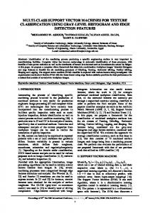
and closeness to the (expected) separating hyperplane should be taken into account in active learning. The SVM active learning approach selects unlabeled documents closest to the classification hyperplane. Although this approach experimentally demonstrated attractive properties, this approach manipulates the distribution of the labeled training documents and might degrade the generalization performance in classifying future unlabeled documents. It is yet unclear that how this manipulation will influence the learning process. However, given a large pool of unlabeled documents, it should be desirable to preserve the density distribution of the ‘pool’ in the learning. Our representative sampling algorithm pursues this idea. It focuses on the uncertain unlabeled documents (e.g. the ones lying within the margin) as other active learning algorithms do and selects representative ones (e.g. cluster centers). As shown in Fig. 1, it guides the learner to concentrate on the most important uncertain data instead of the most uncertain data.

Figure 1. An illustration representative sampling vs. uncertainty sampling for active learning—Unlabeled points selected by representative sampling are the centers of document clusters and preserve the distribution of the pool of data. While uncertainty sampling selects the points, which are the closest to the decision boundary and not relevant to the distribution of documents. (Note: Bold points are support vectors. Dashed lines indicate the Margin. And the solid line is the decision boundary.)

3.3

Orthogonal Subspace Spanning

SVMs have demonstrated state of the art performance in high dimensional domains such as text classification, where the dimensionality may be an order magnitude larger than the number of examples. As indicated by Eq.(2.3.2), the decision boundary is constructed by a subset of the training examples. Typically the subspace spanned by a given set of training examples will cover only a fraction of the available dimensions. One heuristic active learning approach would be to search for examples that are as orthogonal to each other as possible such that a large dimensionality of document

space can be explored. The proposed representative sampling provides such a method. Intuitively, the k-means clustering algorithm detects the subspaces of documents and picks the cluster centers as representatives of the subspaces. Therefore the representative sampling algorithm chooses the uncertain unlabeled examples which also gain most in covered dimensions. 3.4

Version Space Shrinkage

Given a set of labeled training data, there is a set of hyperplanes that correctly separate the data. This set of consistent hypotheses is called the version space [Michell,1982]. Learning problems could be generally viewed as searching the version space to find the in some sense best hypothesis. A reasonable approach is to shrink the version space by eliminating hypotheses that are inconsistent with the training data. Tong and Koller (2001) analyzed the SVM active learning by focussing on the shrinking of the version space and obtained the same algorithm described in [Schohn and Cohn, 2000]. Their discussion is built on the assumption that the data is linearly separable, which, as many experiments have shown is the case for text classification.

(1)

(2)

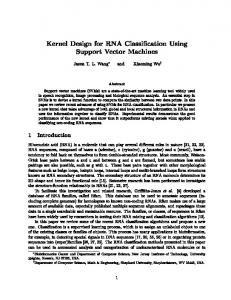
Figure 2. Two examples a and b respectively halve the version space. In the case (1), a and b are two analog examples close to the hyperplane w; while in the case (2), a and b are two orthogonal examples close to the hyperplane w and the combination of them almost quarters the version space. (Note: the center of the inscribed circle is the maximum margin hyperplane.)

Let’s visit Eq. (2.3.2) again. There exists a duality between the input feature pace X and the hyperplane parameter space W : points in X correspond to hyperplanes in W and vice versa. By having this duality, the version space is a region in the parameter space W restricted by support vectors which are hyperphanes in W (see Fig.2). And the decision boundary is the point w within this region (as shown in Fig. 2). Then the maximum margin is interpreted as the maximum distance from the point w to restricting boundaries in W, which correspond support vectors in X. If a new labeled example a =(xa, +1) is observed, then the region w ⋅ x + b < 0 will be eliminated so that a smaller version space is obtained. Therefore adding more labeled

instances can be imagined as using more hyperplanes in W to ‘cut’ and thus decease the version space. In [Tong and Koller, 2001], Lemma 4.3, it was shown that the maximum expected size of the version space over all conditional distributions of y given x can be minimized by halving the version space. It should be noticed that the theory just answered the question of how to select the optimal one unlabeled instance. In [Schohn and Cohn, 2000; Tong and Koller, 2001], the authors implicitly generalized this conclusion to the cases of selecting multi examples without providing a clear justification. It turns out that the issue is more subtle. As illustrated in Fig. 2, two analog examples might lead to non-optimal version space shrinkage, although they both halve the version space. A reasonable heuristic optimization is to divide the version space as equally as possible (as shown in Fig. (2)). This approach is in the same spirit as previous work on SVM active learning and further address the problem of selecting multi unlabeled examples. It can be viewed as a generalization of previous work in [Schohn and Cohn, 2000; Tong and Koller, 2001]. Clustering is a useful approach to identify the optimal clusters such that the inter similarities are minimized and meanwhile the intra similarities are maximized. We use the inner product as the similarity measure, which is exactly the cosine of angle between two x vectors if they have already been normalized to unit length. When the angles between cluster centers (respresented by medoids) are maximized, it is reasonable to believe that the medoid examples evenly divide the version space at the most. Thus our proposed representative sampling provides a straightforward heuristic to optimally choose multi unlabeled examples for active learning.

4 Empirical Study

4.1 Experimental Data Set Table 1 Topics selected for experiments

topic earn acq Money-fx grain crude

Document number 3775 2210 682 573 564

Visibility (%) 36.4 21.3 6.6 5.5 5.3

To evaluate the performance of the proposed representative sampling algorithm we compared it with random sampling and with SVM active learning using uncertainty sampling. We used the Reuters-21578 database, a collection of news documents that have been assigned with one topic, multiple topics or no topic. By eliminating docu-

ments without topics, titles or texts, finally 10369 documents are obtained. Then from these documents, 1000 documents are randomly selected as training set, and another 2000 documents are randomly selected as test set. No overlap exists in the two sets. For text preprocessing, we use the well-known vector space model under the ‘bag of words’ assumption [Salton and McGill, 1983]. The space of the model has one dimension for each word in the corpus dictionary. Finally each document is represented as a stemmed, TFIDF weighted word frequency vector. We use the visibility v to indicate the occurring frequency of a topic in the corpus [Drucker et al., 2001].

v=

nR N

(4.1.1)

where N is the total number of documents in Reuters database; nR is the number of documents with the given topic. As shown in Table 1, we follow the way of [Schohn & Cohn, 2000;Tong and Koller, 2001] and choose 5 most frequently occurring topics for the experiments. We will track the classification performance in cases of different topics.

4.2 Experiment Description and Performance Metrics The purpose of a learner is to train a model (the SVM hyperplane in this work) to identify documents about the desired topic (labeled as “positive”) from the rest documents (labeled as “negative”). To measure the performance of a learner we use a metric of classification accuracy r, which is defined as:

r=

ncorrect N

(4.2.1)

where ncorrect is the number of documents that are classified correctly in test set. N is the total number of documents in test set. We will track the classifier accuracy as a function of labeled training data size for each of the five topics. The proposed representative sampling algorithm will be compared with active learning and random sampling. The experiments of the representative sampling method proceed as the following steps. First, m instances (m/2 positive instances and m/2 negative instances) are randomly selected as “seeds” to train an initial SVM model. At the second step, the instances inside the margin (determined by the SVM model) are clustered into m clusters with the k-means clustering algorithm. Then the instances nearest to each cluster center will be labeled according to their true topic. The learner uses the total cumulated labeled documents so far to rebuild a new model, which is then tested on the independent test set. The same operation is performed in the later iterations. In our experiments the number of iterations is 11, and different value of parameter m (4 and 10) are tested.

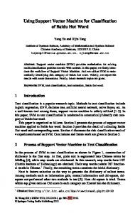
We will run 30 trials for each topic and report the averaged results. Each run of the thirty experiments starts with a set of randomly selected documents. 4.3 Experiment Results and Analysis Figure 3 shows the average value of the test results over five topics (totally 30*5 trails). It shows the classification accuracy r as a function of the total labeled training data size when m=4 and 10. Both the active learning algorithm and the representative sampling algorithms have better performance than the random sampling method, which proves the effectiveness of the active learning strategy using representative sampling and uncertainty sampling. It is observed in Figure 3 that representative sampling significantly outperforms the other two methods in the beginning stages. After a certain number of steps the increase of accuracy of representative sampling is getting slower while the SVM active learning’s accuracy is increasing in a relatively stable manner and finally outperforms representative sampling. The observed results partially conflict with our former expectation and indicate that SVM classifier benefit from clustering only in the initial phase. Figure 4, 5 and 6 show the experimental results for the topics earn, acq and grain, respectively. For the topic earn, the proposed representative sampling shows a very satisfying performance, which is much better than SVM active learning and random sampling. Figure 5 and 6 demonstrate a somewhat similar phenomenon as Figure 3: representative sampling first outperforms SVM active learning but eventually the latter one wins. To clarify this unexpected behavior, we investigate the number of unlabeled instances within the margin. As shown in Figure 7, the number of unlabeled examples within the margin decreases with the representative sampling iterations. If we carefully compare Figure 4, 5, 6 and 7, it is apparent that there exists a strong connection between the accuracy performance of representative sampling and the curves shown in Figure 7. Consider as an example the topic earn: The number of unlabeled instances within the margin decreases consistently and its accuracy also consistently outperforms other two methods. For the example of topic arc or grain, one the other hand, the size of unlabeled data within the margin decreases quickly at the beginning but later decreases only slowly. In comparison, accuracy increases quickly at first but then increases only slowly. The observed phenomenon might be interpreted as follows. If SVM learning progresses well, then the number of unlabeled data within the margin drops quickly. Thus the size of unlabeled data within the margin is a good indicator for the performance of the SVM. In particular, representative sampling performs badly if there is no clear cluster structure in those data. A good hybrid approach might be to start with representative sampling and to switch to normal active learning at an appropriate instance. This instance can be defined experimentally by observing the change in the number of unlabeled data within the margin. Figure 8 shows the initial result of such a hybrid algorithm applied to the topic acq. As shown, the strategy switches from representative sampling to active learning at the correct instance.

Finally we would like to emphasize that achieving a good performance in initial stages is an important feature for text classification since experts always expect the quality of a classification system by the initial interaction.

(a)

(b)

Figure 3. Average classification accuracy r of five topics versus the number of labeled training instances, (a) m=4 (b) m=10

(a)

(b)

Figure 4. Average classification accuracy r for topic earn versus the number of labeled training instances, (a) m=4 (b) m=10

(a)

(b)

Figure 5. Average classification accuracy r for topic acq versus the number of labeled training instances, (a) m=4 (b) m=10

(a)

(b)

Figure 6. Average classification accuracy r for topic grain versus the number of labeled training instances, (a) m=4 (b) m=10

(a) (b) Figure 7. Average number of the uncertain instances in the margin for three topics versus the number of labeled training instances, (a) m=4 (b) m=10

(a) (b) Figure 8. Average classification accuracy r for topic earn versus the number of labeled training instances, with the hybrid method (a) m=4 (b) m=10

5 Conclusions This paper made the attempt to investigate the value of the unlabeled data distribution, e.g. clustering structure, in SVM active learning and proposed a novel active learning heuristic for text classification. In addition, a novel hybrid strategy was presented. The analysis about optimal multi-instance selection for version space shrinkage provides a novel extension to previous work. The experiments demonstrated that in the beginning stages of active learning, the proposed representative sampling approach significantly outperformed SVM active learning and random sampling. This is a favorable property for the applications to text retrieval. However, in some cases SVM, active learning after a number of active learning iterations outperformed the representative sample. We initially analyzed the reasons for this phenomenon and found that the number of unlabeled instances within the SVM margin is a good indicator for the performance of our approach. The poor performance of representative sampling in some cases might be due to the poor clustering structure and high complexity of unlabeled data within the margin. This observed problem attracts us to further study the relation between data distribution within the margin and the performance of SVM in text classification tasks. Also, the work we described here is somewhat heuristic, but might provide a good starting point for further refinement towards a solid learning approach in future work.

References 1. Blum, A., Mitchell, T.: Combining Labeled and Unlabeled Data with Co-training. In Proceedings of the Eleventh Annual Conference on Computational Learning Theory, (1998) 92-100 2. Burges, C.J.: A tutorial on support vector machines for pattern recognition. Data Mining and Knowledge Discovery 2, (1998) 121-167 3. [Drucker et al., 2001] H. Drucker, B. Shahrary and D.C. Gibbon, Relevance feedback using support vector machines. Proc. 18th International Conf. On Machine Learning, 122-129, 2001. 4. Fishman, G.: Monte Carlo. Concepts, Algorithms and Applications. Springer Verlag, 1996 5. Gray, R.M., Vector Quantization, IEEE ASSP Magazine, (1984) 4--29. 6. Joachims, T.: Text Categorization with Support Vector Machines: Learning with Many Relevant Features. In European Conference on Machine Learning, ECML-98, (1998), 137142 7. Joachims, T.: Transductive Inference for Text Classification using Support Vector Machines. In Proceedings of International Conference on Machine Learning, (1999) 8. Lewis, D., Gale, W.: A Sequential Algorithm for Training Text Classifiers. Proc. of the Eleventh International Conference on Machine Learning. Morgan Kaufmann, (1994) 148156 9. McCallum, A., Nigam, K.: Employing EM in pool-based active learning for text classification. In Proceedingsof the fifteenth international conference of machine learning (ICML 98), (1998) 350-358 10. Mitchell, T.: Generalization as search. Artificial Intelligence 28 (1982) 203-226 11. Platt, J.: Probabilistics for SV Machines. In Advances in Large Margin Classifiers. A.Smola, P. Bartlett, Bscholkopf, D. Shuurmans eds., MIT Press (1999) 61-74

12. Schohn, G., Cohn, D.: Less is More: Active Learning with Support Vector Machines. Proc. of the Seventeenth International Conference on Machine Learning (2000) 13. Seung, H.S., Opper, M., Sompolinsky, H.: Query by committee. In Proceedings of the fifth annual ACM workshop on Computational Leanring Theory, (1992), 287-294 14. Tong, S., Koller, D.: Support Vector Machine Active Learning with Applications to Text Classification. Journal of Machine Learning Research. Volume 2, (2001) 45-66 15. Vapnik, V.: Estimation of Dependences Based on Empirical Data. Springer Verlag. 1982. 16. Zhang, T., Oles, F.: A probabilistic analysis on the value of unlabeled data for classification problems. International Conference on Machine Learning (2000)