Evaluations of the validation methods were based on the analysis results compared to ... and their sensitivity to the discrepancy between sets of data and 2) to ...
REVIEW OF CORRELATION METHODS FOR EVALUATING FINITE ELEMENT SIMULATIONS OF IMPACT INJURY RISK Qian Wang, Hampton C. Gabler Virginia Tech-Wake Forest, Center for Injury Biomechanics Blacksburg, VA 24061
ABSTRACT Finite element models have been used to understand human injury responses in various crash configurations. Most of the model validations were limited to qualitative descriptions. Quantitative analysis was needed for the validation of finite element models against experimental results. The purpose of this study is to compare the existing correlation techniques and to determine the best method to use for evaluating finite element simulations of impact injury risk in vehicle crashes. Five correlation methods in the literature were reviewed for systematic comparisons between simulations and tests. A full frontal impact test of a 1997 Geo Metro was simulated. The finite element model of a 1997 Geo Metro was obtained from NCAC finite element model archive. The acceleration and velocity responses of the vehicle seat were extracted from the simulation and compared to the test data. Evaluations of the validation methods were based on the analysis results compared to the suggested criteria. Performance of the different methods showed that the Comprehensive Error Factor method was the best overall correlation method, and therefore was recommended for assessing occupant injury potentials in vehicle accidents. Keywords: Correlation Method, Finite Element, Frontal Impact
INTRODUCTION Mathematical models have been used extensively in injury biomechanics to investigate occupant injury responses in vehicle crashes, especially when experiments are difficult to conduct. To ensure the reliability of these models for injury response prediction, the models must first be validated against any available experimental data. However, mathematical model validations against experimental results in most papers are limited to qualitative descriptions, which generally focus on generally appearance characteristics of the responses. Due to the impreciseness of these descriptions, it is difficult to use them for systematic evaluations. Quantitative methods are needed to determine the level of model validation against the experiments. This paper evaluates several quantitative validation methods in the existing literature that assess the discrepancy between a measured and a simulated transient response history.
METHODS The purpose of this paper is 1) to compare the existing correlation methods according to their simplicity and their sensitivity to the discrepancy between sets of data and 2) to suggest the most appropriate correlation method for evaluating finite element simulations of impact injury risk in vehicle crashes. The following five quantitative correlation techniques were reviewed in this paper. 1. Comprehensive Error Factor: Comprehensive Error Factor method assigns a single numerical value to the discrepancy between two time histories over a defined period. The difference between two data sets is described by magnitude, phase, and comprehensive error factors [1]. It was suggested by the author that the two responses were in good agreement if the comprehensive error factor was less than 20 %. To compare a calculated time history c(t) and the corresponding measured response m(t), three functions Φ c 2 , Φ m 2 , and Φcm are computed and shown in Equation 1:
t
Φ c2 ( t, τ) = ∫0 c 2 ( t + τ)dt t 0
Φ m 2 ( t , τ) = ∫ m ( t )dt 2
, Φ cm ( t , τ) = ∫0t c( t + τ) m( t )dt
(eq.1)
where τ is the uncertain delay between starting times for the two responses. Calculations of two correlation functions G(t, τ) and H(t, τ) are shown in Equation 2. ⎛ Φ 2 ( t , τ) ⎞ ⎟ G ( t , τ) = ⎜ c ⎜ Φ 2 ( t ,0) ⎟ ⎝ m ⎠
1/ 2
⎛ ⎞ Φ cm ( t , τ) ⎟ , H( t , τ) = ⎜ ⎜ Φ 2 ( t , τ)Φ 2 ( t ,0) 1 / 2 ⎟ m ⎝ c ⎠
[
1/ 2
]
(eq.2)
As shown in Equation 2, G(t, τ) is sensitive to magnitude difference between c(t) and m(t), but is not sensitive to phase discrepancy between the two. Contrarily, H(t, τ) is sensitive to phase discrepancy, but is not sensitive to magnitude discrepancy. Finally, the magnitude factor Em, phase factor Ep, and comprehensive factor Ec can be calculated by Equation 3.
E m (τ) = G ( t , τ) − 1 E p (τ) = 1 − H( t, τ)
[
2
2
, E c (τ) = E m (τ) + E p (τ)
]
1/ 2
(eq.3)
2. Normalized Integral Square Error (NISE) Method: Normalized Integral Square Error (NISE) method is another measure to quantify the difference between two time histories over their duration. NISE method considers phase shift, amplitude difference, and shape difference [2]. To compute the NISE for two discrete time histories c(t) and m(t), four correlation functions are defined and expressed in Equation 4: 1 N 1 N ∑ (c i ( t )m i ( t )) Ryy(0) = ∑ (m i ( t )m i ( t )) N i =1 N i =1 , N 1 1 N−n Rxx (0) = ∑ (c i ( t )c i ( t )) Rxy(τ) max = ∑ (c i ( t )m i + n ( t )) N i =1 N − n i =1
Rxy(0) =
(eq.4)
where N is the number of data points in each curve, τ is the time delay that maximizes function Rxy(τ), n is the time shift index and is equal to τ divided by the constant time step. The portions of the NISE due to phase shift, amplitude difference, and shape difference are defined by Equation 5. The total NISE is the sum of the three portions of NISE.
2Rxy(τ) max 2Rxy(0) − Rxx (0) + Ryy(0) Rxx (0) + Ryy(0) Rxy(τ) max 2Rxy(τ) max − NISE(Amplitude) = Rxx (0)Ryy(0) Rxx (0) + Ryy(0)
NISE(Phase) =
NISE(shape) = 1 −
(eq.5)
Rxy(τ) max Rxx (0)Ryy(0)
3. Cumulative Variance Method: Cumulative Variance method quantifies the discrepancy between two sets of data by computing their sum of squared errors [3]. If the simulation results follow the test data exactly, the cumulative variance equals zero. It was noted in the paper that a cumulative variance of 25000 or less implied good correlation between the two data sets. Equation 6 is used to
evaluate two discrete time histories c(t) and m(t). τ is the time delay between the two curves that minimizes CV in Equation 6, where i is the data point index number. CV = ∑ [c i ( t ) − m i ( t − τ)] N
2
(eq.6)
i =1
4. The Numerical Analysis of Roadside Design (NARD) validation parameters: The NARD correlation method involves the calculation of correlation coefficient and nth relative difference of moments between two time history curves [4]. The correlation coefficient is a measurement of degree of linear relationship between two time histories. The correlation factor should be greater than 0.95. This indicates that the signal can be linearly transformed to match the reference signal. It is possible and quite common to have a very good correlation factor and still have significant scaling and bias errors. The relative moments describe the characteristics of the time history curves. The 0th, 1st, and 2nd moments correspond to the area under the curve, area moment of the curve, and area moment of inertia of the curve, respectively. The two signals are considered equivalent if the 0th through 5th Moments of the residual are less than 20%. The correlation coefficient is given by Equation 7. c and m are the mathematical means of the two time history curves.
∑ [(c i ( t ) − c )(m i ( t ) − m)] N
CorrelationCoefficient =
i =1 N
N
(eq.7)
∑ (c i ( t ) − c ) ∑ ( m i ( t ) − m )
i =1
2
2
i =1
The relative nth moments of two time histories c(t) and m(t) are expressed in Equation 8. The relative difference of the moments can be calculated in Equation 9, where ∆t is the constant time step. N
Moment (c( t )) = n r
∑ t i c i ( t ) Δt
N
n
i =1
N ⎛∑ ⎞ ⎜ ti ⎟ ⎝ i =1 ⎠
n +1
, Moment (m( t )) = n r
∑ t i m i ( t ) Δt n
i =1
N ⎛∑ ⎞ ⎜ ti ⎟ ⎝ i =1 ⎠
n +1
The Re lativeDifferenceOfMoments(ε) = Moment nr (c( t )) − Moment nr ( m( t ))
(eq.8)
(eq.9)
5. The Analysis of Variance (ANOVA) Method: The ANOVA method is a statistical test of the residual error between two signals [5]. A two-tailed t-test is conducted to determine if there is significant difference between the two time histories at the specified level of significance. The suggested critical t-statistic is 2.58 or less. The potential problem for the t-statistic is that highly correlated signals will fail the t-statistic test due to slight but consistent bias or phase errors. The tstatistic is defined by Equation 10: T=
e
(eq.10) σe / n where e is average residual between the two curves, σe is standard deviation of the residuals, and n is the number of paired samples. To compare the five correlation methods, the results of a full frontal barrier test of a 1997 Geo Metro with the corresponding results of a LS-DYNA finite element simulation on this crash test were used. The acceleration and velocity responses of the vehicle in the simulation and the crash test were
compared using the above correlation methods. The finite element model of a 1997 Geo Metro developed by the National Crash Analysis Center (NCAC) was used in this study. A full frontal barrier Test 2239 of Geo Metro of model year 1995 was obtained from the NHTSA crash database.
RESULTS The acceleration and velocity responses of vehicle seats were extracted from the FE model and compared to the crash test results. The time step size of the finite element simulation was 1.33*10-6 s. All data were filtered with a frequency of 60 Hz. The acceleration and velocity comparisons of the Geo Metro full frontal barrier test are shown from Figure 1 to Figure 4. A spike with a peak value of 50 G’s was observed at around 0.03 s in the acceleration responses of vehicle seats in Test 2239. However, no acceleration response with similar magnitude was observed in the simulation. The comparisons of vehicle seat velocity showed that the test and simulation had the comparable rebound velocity. The main difference between the results was a time delay of the overall velocity response in the simulation.
Figure 1. Left rear seat acceleration in x direction.
Figure 2. Right rear seat acceleration in x direction.
Figure 3. Left rear seat velocity in x direction.
Figure 4. Right rear seat velocity in x direction.
Comparisons of the test and model using each of the different correlation methods are given in Table 1. The shading indicates that the computed correlation factors meet the suggested criteria. A time shift, which was the generally uncertain delay between starting time for the two time histories, was calculated for the first three correlation methods. The phase errors in the acceleration and velocity responses of the left seat in x direction were examined. The aligned curves are shown in Figure 5 and Figure 6. Comparisons between the test and simulation by using the Comprehensive Error Factor method showed that the delay in the simulation responses accounted for the majority of comprehensive errors. The overall difference between the test and simulation results was about 2.5 % and 0.1 % for the acceleration
and velocity responses respectively, which was well below the suggested criterion of 20 %. It was also noted in the table that the time shift needed to align the curves are very comparable. Analysis by the NISE method showed that time shift errors were found between otherwise similar curves. However, the NISE method failed to identify the phase shifts for the velocity responses. Results from the assessment by the Cumulative Variance method demonstrated that the acceleration responses exceed the criterion of 25000 while the vehicle velocity histories correlated well with each other. The NARD evaluation criteria and Analysis of Variance method were also used to determine if the simulation accurately replicated the test. The results obtained from the NARD analysis showed that only three relative differences of moments met the criterion of 0.2 for acceleration responses and nine velocity history comparisons exceeded the criterion. Contradictory to the findings of the relative difference of moments, the correlation factors indicated that the velocity curves had very good correlation while the acceleration histories failed to meet the standard of 0.95. Finally, the evaluation by Analysis of Variance method showed that the acceleration responses were highly related. The t-statistics showed that there was statistically significant difference between the velocity curves.
Figure 5. Aligned left rear seat acceleration in x direction.
Figure 6. Aligned left rear seat velocity in x direction.
Table 1. Dynamic response comparisons between Test 2339 and simulation by different correlation methods. Comparison Parameters Magnitude Difference (%) Comprehensive Phase Difference (%) Error Factor Comprehensive Factor (%) Time Shift (s) Phase Difference (%) Amplitude Difference (%) NISE Shape Difference (%) Total Difference (%) Time Shift (s) CV Cumulative Variance Time Shift (s) 0th Moment Difference (%) 1st Moment Difference (%) 2nd Moment Difference (%) NARD 3rd Moment Difference (%) 4th Moment Difference (%) 5th Moment Difference (%) Correlation Factor t-statistic Analysis of Variance
Left Seat A -0.50 2.42 2.47 0.0118 53.68 0.03 -42.73 10.98 0.0107 73384 0.0107 0.7 21.2 37.9 58.3 88.1 138.1 0.890 0.41
Right Seat A -0.57 2.73 2.79 0.0128 59.37 0.01 -41.00 18.38 0.0117 94082 0.0118 2.2 17.7 30.6 43.1 59.1 84.1 0.816 0.99
Left Seat V 0.017 0.095 0.097 0.0108 45.81 1.09 -44.84 2.05 0.0000 900 0.0104 24.1 69.2 333.4 47.5 23.0 13.3 0.987 46.26
Right Seat V -0.027 0.0999 0.10 0.0126 45.58 1.42 -44.18 2.82 0.0000 1333 0.0122 28.1 78.3 2444.2 90.4 49.9 36.4 0.981 48.87
DISCUSSION The differences between the test data and simulation results were evaluated by five correlation methods. Some potential problems were found for these correlation methods. The time delay in the simulation was not detected by the NISE method. Further improvements in the correlation algorithm may be needed. The Cumulative Variance method provides a simple error measure for evaluating the difference between responses. However, the correlation calculation, which is based on the sum of squared errors, could also indicate that a small number of large differences might exceed the criteria whereas a large number of small differences may meet the criteria. The NARD analysis showed that the criterion of 0.2 was stricter for higher order of relative difference of moments. Although there were obvious time delay between the vehicle seat velocities in the simulation and the test data, the calculated correlation factors suggested that the responses were highly related. The ANOVA method was used to determine the significant difference between two time histories by computing the t-statistics. The results indicated a good correlation between the acceleration responses despite the large number of small differences. Whereas the velocity time histories failed to meet the criteria due to the large phase errors between otherwise similar curves.
CONCLUSIONS This paper reviewed the five existing correlation methods for evaluating finite element simulations of impact injury risk in vehicle crashes. The analysis from Comprehensive Error Factor method showed that this method could be considered as a candidate for quantitatively estimating the fit between two responses. The NISE method also divided the total error into three portions. However, the comparisons of vehicle velocity responses revealed some possible defects in its validation algorithms. The assessment by the Cumulative Variance method showed that it was sensitive to the magnitude discrepancy between two histories although it was unaffected by the time delay between two curves. Another potential problem of the Cumulative Variance method is that the calculation could indicate that a small number of large differences might exceed the criteria whereas a large number of small differences may meet the criteria. The analysis results obtained from the NARD method demonstrated that the frequently occurred phase shift errors accounted for the inconsistencies in the results between relative difference of moments and correlation factors. Similarly, the t-statistics calculated in the ANOVA method was unable to determine the error caused by time delay between two otherwise similar time histories. In conclusion, the Comprehensive Error Factor method showed the best performance in the signal comparisons. Therefore, it was chosen and recommended as the correlation method for evaluating finite element simulations of impact injury potential in motor vehicle accidents.
REFERENCES [1] T. L. Geers, “An objective error message for the comparison of calculated and measured transient response histories,” The Shock and Vibration Bulletin, June, 1984. [2] J. Jovanovski, “Crash data analysis and model validation using correlation techniques,” Proceedings of the SAE International Congress and Exposition, Detroit, Michigan, USA, SAE 810471, 1981. [3] R. M. Morgan, J. H. Marcus, and R. H. Eppinger, “Correlation of side impact dummy-cadaver tests,” Proceedings of the 25th Stapp Car Crash Conference, San Francisco, California, USA, 1981. [4] S. Basu, and A. Haghighi, “Numerical analysis of roadside design (NARD) Volume III: Validation procedure manual,” Report No. FHWA-RD-88-213, Federal Highway Administration, September, 1988. [5] M. H. Ray, “Repeatability of full-scale crash tests and a criteria for validating simulation results,” Transportation Research Record 1528, TRB, National Research Council, Washington, DC, 1996.