Rhythmic Auditory Cortex Activity at Multiple ... - Semantic Scholar

7750 • The Journal of Neuroscience, May 20, 2015 • 35(20):7750 –7762

Systems/Circuits

Rhythmic Auditory Cortex Activity at Multiple Timescales Shapes Stimulus–Response Gain and Background Firing Christoph Kayser,1 Caroline Wilson,2 X Houman Safaai,3 Shuzo Sakata,2* and Stefano Panzeri3* 1

Institute of Neuroscience and Psychology, University of Glasgow, Glasgow, G12 8QB, 2Strathclyde Institute of Pharmacy and Biomedical Sciences, University of Strathclyde, Glasgow, G1 1XQ, United Kingdom, and 3Neural Computation Laboratory, Center for Neuroscience and Cognitive Systems, Istituto Italiano di Tecnologia, I-38068 Rovereto, Italy

The phase of low-frequency network activity in the auditory cortex captures changes in neural excitability, entrains to the temporal structure of natural sounds, and correlates with the perceptual performance in acoustic tasks. Although these observations suggest a causal link between network rhythms and perception, it remains unknown how precisely they affect the processes by which neural populations encode sounds. We addressed this question by analyzing neural responses in the auditory cortex of anesthetized rats using stimulus–response models. These models included a parametric dependence on the phase of local field potential rhythms in both stimulus-unrelated background activity and the stimulus–response transfer function. We found that phase-dependent models better reproduced the observed responses than static models, during both stimulation with a series of natural sounds and epochs of silence. This was attributable to two factors: (1) phase-dependent variations in background firing (most prominent for delta; 1– 4 Hz); and (2) modulations of response gain that rhythmically amplify and attenuate the responses at specific phases of the rhythm (prominent for frequencies between 2 and 12 Hz). These results provide a quantitative characterization of how slow auditory cortical rhythms shape sound encoding and suggest a differential contribution of network activity at different timescales. In addition, they highlight a putative mechanism that may implement the selective amplification of appropriately timed sound tokens relative to the phase of rhythmic auditory cortex activity. Key words: delta rhythm; information coding; LNP models; network state; neural coding; receptive fields

Introduction Accumulating evidence suggests that low-frequency rhythms play an important role for hearing (Schroeder and Lakatos, 2009; Giraud and Poeppel, 2012; Leong and Goswami, 2014). Neuroimaging and intracranial recordings show that neural activity in the auditory cortex (A1) at frequencies below ⬃12 Hz entrains to the temporal structure of sounds and carries information about

Received Jan. 21, 2015; revised March 17, 2015; accepted April 7, 2015. Author contributions: C.K., S.S., and S.P. designed research; C.K., C.W., and H.S. performed research; C.K., C.W., S.S., and S.P. contributed unpublished reagents/analytic tools; C.K., H.S., and S.P. analyzed data; C.K., S.S., and S.P. wrote the paper. The initial stages of this work were supported by the Max Planck Society (C.K.) and were part of the research program of the Bernstein Center for Computational Neuroscience (Tu¨bingen, Germany) funded by the German Federal Ministry of Education and Research (FKZ 01GQ1002; C.K. and S.P.). The work was also supported by the Action on Hearing Loss (“Flexi Grant”; to C.K.), Medical Research Council Grant MR/J004448/1 (to S.S.), the SI-CODE Project of the FP7 of the European Commission (FET-Open, Grant FP7-284553; to S.P.), and the Autonomous Province of Trento (“Grandi Progetti 2012,” the “Characterizing and Improving Brain Mechanisms of Attention–ATTEND” project; to S.P.). We are grateful to N. K. Logothetis and R. Brasselet for collaborations in previous phases of this work. *S.S. and S.P. contributed equally to this work. The authors declare no competing financial interests. This article is freely available online through the J Neurosci Author Open Choice option. Correspondence should be addressed to C. Kayser, Institute of Neuroscience and Psychology, University of Glasgow, 58 Hillhead Street, Glasgow G12 8QB, UK. E-mail: [email protected]. C. Wilson’s present address: Medical Research Council Institute of Hearing Research Nottingham, University of Nottingham, University Park Nottingham, NG7 2RD, UK. DOI:10.1523/JNEUROSCI.0268-15.2015 Copyright © 2015 Kayser et al. This is an Open Access article distributed under the terms of the Creative Commons Attribution License Creative Commons Attribution 4.0 International, whichpermitsunrestricteduse,distributionandreproductioninany medium provided that the original work is properly attributed.

sound identity (Kayser et al., 2009; Szymanski et al., 2011; Ding and Simon, 2012, 2013; Ng et al., 2013), possibly because natural sounds contain important acoustic structures at these frequencies (Ding and Simon, 2013; Doelling et al., 2014; Gross et al., 2013). Importantly, the degree of rhythmic entrainment correlates with perceptual intelligibility (Mesgarani and Chang, 2012; Doelling et al., 2014; Peelle et al., 2013), linking the timescales relevant for acoustic comprehension with those of neural activity (Rosen, 1992; Ghitza and Greenberg, 2009; Zion Golumbic et al., 2012). Based on these results, it has been hypothesized that slow rhythmic activity in the A1 reflects key mechanisms of sound encoding that have direct consequences for hearing (Giraud and Poeppel, 2012; Peelle and Davis, 2012; Strauß et al., 2014b). This raises the central question of how precisely rhythmic auditory cortical activity shapes sensory information processing. Electrophysiological recordings showed that slow rhythms reflect fluctuations in cortical excitability (Bishop, 1933; Azouz and Gray, 1999; Womelsdorf et al., 2014; Pachitariu et al., 2015; Reig et al., 2015) and the strength of neuronal firing (Lakatos et al., 2005; Belitski et al., 2008; Haegens et al., 2011). Such intrinsic excitability changes could either simply reflect stimulus-unrelated modulations of background firing or could reflect a profound influence of cortical dynamics on the sensory computations by individual neurons. Indeed, a prominent theory suggests that auditory network rhythms help to selectively amplify the encoding of acoustic inputs that are aligned appropriately with the phases of network excitability captured by these rhythms

Kayser et al. • LFP-Dependent Stimulus Encoding in Auditory Cortex

(Schroeder and Lakatos, 2009; Lakatos et al., 2013). However, whether and how precisely network activity affects the computations by which auditory neurons represent sensory inputs remains unknown. To directly investigate this relationship, we recorded spiking activity and local field potentials (LFPs) in the rat primary auditory cortex (A1) during acoustic stimulation and epochs of silence. We developed linear–nonlinear Poisson (LNP) models that included, besides a static stimulus–response tuning [spectrotemporal receptive fields (STRFs)], parameters for sensory gain and stimulus-unrelated background activity that varied with the state of network activity as indexed by the phase or power of LFPs at different timescales. Using these models, we uncovered that including a systematic dependence on LFP phase of both background activity (prominent for delta, 1– 4 Hz) and of stimulus– response gain (prominent between 2 and 12 Hz) improved response prediction. These results highlight mechanisms by which systematic changes in stimulus–response transfer could selectively amplify or attenuate responses at specific phases of network rhythms and provide a possible neural underpinning for rhythmic sensory selection and perception (Vanrullen et al., 2011; Giraud and Poeppel, 2012; Jensen et al., 2012).

Materials and Methods General procedures and data acquisition. Recordings were obtained from six adult Sprague Dawley rats (males, 253–328 g). Experiments were performed in accordance with the United Kingdom Animals (Scientific Procedures) Act of 1986 and were approved by the United Kingdom Home Office and the Ethical Committee of Strathclyde University. The general procedures followed those used in previous work (Sakata and Harris, 2009). The animals were anesthetized with 1.5 g/kg urethane, and lidocaine (2%, 0.1– 0.3 mg) was administered subcutaneously near the site of incision. Body temperature was maintained at 37°C using a feedback temperature controller. To facilitate acoustic stimulation, a head post was fixed to the frontal bone using bone screws, and the animal was placed in a custom head restraint that left the ears unobstructed. Recordings took place in a single-walled soundproof box (MAC-3l IAC Acoustics). After reflecting the left temporalis muscle, the bone over the left A1 was removed and a small duratomy was performed. A 32-channel silicon tetrode probe (A8x1-tet-2mm-200-121-A32; NeuroNexus Technologies) was inserted slowly (⬍2 ␮m/s) into infragranular layers of A1 using a motorized manipulator (DMA-1511; Narishige). During recording, the brain was covered with 1% agar/0.1 M PBS to reduce pulsation and to keep the cortical surface moisturized. Recordings started after a waiting period of ⬃30 min. Broadband signals (0.07 Hz to 8 kHz) were amplified (1000 times) using a Plexon system (HST/32V-G20 and PBX3) relative to a cerebellar bone screw and were digitized at 20 kHz (PXI; National Instruments). Acoustic stimuli were generated through a multi-function data acquisition board (NI-PCI-6221; National Instruments) and were presented at a sampling rate of 96 kHz using a speaker driver (ED1; Tucker-Davis Technologies) and using free-field speakers (ES1; Tucker-Davis Technologies) located ⬃10 cm in front of the animal. Sound presentation was calibrated using a pressure microphone (PS9200KIT-1/4; ACO Pacific) to ensure linear transfer and calibrated intensity. For this study, a series of naturalistic sounds was presented. These sounds were obtained from previous work (Kayser et al., 2009) and reflect various naturalistic noises or animal calls that were recorded originally in the spectral range of 200 Hz to ⬃15 kHz. For this study, they were shifted into the rat’s hearing range by resampling to cover frequencies up to ⬃30 kHz (for a spectral representation, see Fig. 1A). The stimulus sequence lasted 30 s and was presented at an average intensity of 65 dB rms and was repeated usually 50 times during each experiment with an interstimulus interval of up to 5 s. We also recorded spontaneous activity before the sound presentation for a period of 250 s. Neural signals were processed as follows. Spike detection for each tetrode took place offline and was performed with freely available software (EToS

J. Neurosci., May 20, 2015 • 35(20):7750 –7762 • 7751

version 3; http://etos.sourceforge.net; Klusters, http://klusters.sourceforge.net; Hazan et al., 2006; Takekawa et al., 2010), using exactly the standard parameters described in previous studies (Takekawa et al., 2010). Broadband signals were high-pass filtered, spikes were detected by amplitude thresholding, and potential artifacts were removed by visual inspection. We recorded reliable spiking activity from n ⫽ 38 sites (of 48 sites in total) and analyzed this as multiunit activity (MUA). We also performed clustering with the Klusters software and isolated single units based on a spike isolation distance of ⬎20 (Schmitzer-Torbert et al., 2005). However, the overall spike rate of single units in this preparation was low (mean response during stimulation of 1.9 ⫾ 0.3 spikes/s; mean ⫾ SEM across units) and hence did not allow us to perform on the LFPdependent analysis described below on single-unit activity because of undersampling of the response space. Hence, we restrict the present report to MUA data. For every recording site, field potentials were extracted from the broad-band signal after resampling the original data to 1000 Hz sample rate and were averaged across all four channels per tetrode. A Kaiser finite impulse response filter (sharp transition bandwidth of 1 Hz, pass-band ripple of 0.01 dB, and stop-band attenuation of 50 dB; forward and backward filtering) was used to derive band-limited signals in different frequency bands (for details, see Kayser, 2009). Here we focused on the following overlapping bands, [0.25–1], [0.5–2] and [1– 4] Hz and continuing in 4-Hz-wide bands up to 24 Hz. The instantaneous power and phase of each band was obtained from the Hilbert transform. To relate spike rates and stimulus encoding to the phase or power of each bandlimited signal, we labeled each spike with the respective parameter recorded from the same electrode at the time of that spike (Kayser et al., 2009). For phase, this was achieved by using equally spaced bins covering the 2␲ cycle. For power, we divided the range of power values observed on each electrode into equally populated bins. For the results reported here, we used four bins, but using a higher number (e.g., eight bins) did not change the results qualitatively. We focused on frequencies ⬍24 Hz because preliminary tests had revealed that modulations of firing rates were strongest at low frequencies. Terminology and assessment of cortical states. The term cortical state is used in the literature to describe a wide range of phenomena, with intrinsically different timescales, but usually varying on the scale of hundreds of milliseconds or longer (Curto et al., 2009; Harris and Thiele, 2011; Marguet and Harris, 2011; Sakata and Harris, 2012; Pachitariu et al., 2015). An example is a transition between the synchronized or desynchronized (also up/down) states. These slow and relatively widespread network state transitions are likely different from the more rapid changes in network excitability indexed by the phase or power of LFP bands ⬎0.5 Hz (Canolty and Knight, 2010; Panzeri et al., 2010; Haegens et al., 2011; Lakatos et al., 2013). To distinguish these two timescales of network properties, here we use the term “cortical state” for properties of network dynamics on scales of seconds or longer (such as the synchronized and desynchronized states that can be detected from the LFP spectrum) and use the term LFP state to denote cortical dynamics indexed by the power or phase of different LFP bands, which persist on shorter timescales. This nomenclature is conceptually similar to that of Curto et al. (2009), who distinguished between “dynamic states” of cortex referring to properties of network dynamics on a timescale of seconds or more and “activity states” describing cortical states that persist on shorter timescales of few tens to few hundred milliseconds. We quantified cortical state using the ratio of low-frequency (0.25–5 Hz) LFP power divided by the total LFP power (0.25–50 Hz) and using the correlation of firing rates across distant electrodes (Curto et al., 2009; Sakata and Harris, 2012; Pachitariu et al., 2015). These measures were correlated across sessions and times, and, when plotted over the experimental time axis, they both indicated that cortical states were stable for all but one of six experiments (Experiment 1), during which we observed more pronounced variations in LFP power ratio than for the others (see Fig. 6A, black). They also indicate that the results here were obtained during synchronized states (Curto et al., 2009). We note, as discussed in Results (see Fig. 6), that we observed the same main findings in each of the experiments, demonstrating that slight variations in cortical state

Kayser et al. • LFP-Dependent Stimulus Encoding in Auditory Cortex

7752 • J. Neurosci., May 20, 2015 • 35(20):7750 –7762

A

B

Frequency [kHz]

0

Phase bin 1st 2nd 3rd 4th 1-4Hz

Trials

10 20 30

C

5

Stimulus

10

15

Spontaneous

20

25

30

% Rate Modulation 0

30

60

D

60

Spontaneous Stimulus

1

% Spikes / bin

Frequency [Hz]

0.25

Time [s]

Trials

40 0

4 8 12 16 20

40

20

0 1st 2nd 3rd 4th

Phase bin

10

40

Phase bin

% Spikes/bin

0

0.5

1

1.5 Time [s]

2

2.5

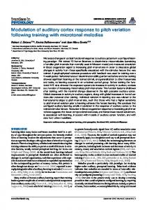
3

Figure 1. Phase dependence of auditory cortical responses during acoustic stimulation and spontaneous activity. A, Spectrotemporal representation of the acoustic stimulus sequence. Red (blue) colors indicate high (low) sound intensity. B, Example data from one site showing the phase of the delta band (1– 4 Hz) with LFP color coded (top), the spike raster across multiple trials (middle), and the trial-averaged firing rate (bottom). In the raster, each spike is colored with the delta phase at the time of spike. C, Left and middle, Distribution of firing rates across LFP phase bins for different frequency bands during stimulation and spontaneous activity. Color codes are the average across units (n ⫽ 38). Right, Modulation of firing rate. D, Distribution of spikes per phase bin for the delta band. Error bars denote mean and SEM across units. across sessions did not confound with our results pertaining to the more rapid network dynamics indexed by LFP phase. Quantification of LFP state-dependent firing rates and circular phase statistics. To quantify the relation between spikes and LFP phase (or power), we calculated the percentage of spikes elicited in each phase (or power) bin. The “firing rate modulation” with phase was calculated as the firing rate in the preferred bin (i.e., the bin with maximal rate) minus that in the opposing bin (i.e., the bin 180° apart). Using the difference between maximal and minimal firing rate across bins (Montemurro et al., 2008) yielded results very similar to those presented here. For power, the rate modulation was defined as the value in the highest power bin minus that in the lowest. We defined the “preferred phase” for each unit as the circular average of the phase at all spikes. Statistical tests for the nonuniformity of the spike-phase distribution were computed with the Rayleigh’s test for non-uniformity of circular data. STRFs and response models. To model the neural input– output function, we used LNP models, schematized in Figure 2A. These models are made of a linear filter characterizing the selectivity of each unit in time and sound-frequency domains (the STRF) and of a nonlinear stimulus– response transfer function translating the stimulus filter activation into a corresponding spike rate (Fig. 2A). We extended this basic model to describe the time-dependent spike rate q(t) as the sum of a stimulusinduced component qstim(t) plus an additive component b that models the presence of ongoing and stimulus-unrelated background firing. In more detail, for each unit, the STRF was obtained using regularized regression based on the data recorded during stimulus presentation (Machens et al., 2004; David et al., 2007) and by correcting for the temporal autocorrelation inherent to natural sounds (Theunissen et al., 2001). A time–frequency representation of the stimulus was obtained by resampling sounds at 90 kHz and deriving a time–frequency representation using sliding window Fourier analysis (the spectrogram function in MATLAB) based on 100 ms time windows, at 5 ms nominal temporal resolution and by selecting logarithmically spaced frequencies (eight steps per octave) between 800 Hz and 43 kHz. The square root of the power-spectral density was used for the STRF analysis. STRFs were calculated based on single-trial responses using ridge regression, introducing two additional constraint parameters for filter smoothness and sparseness (for details, see Machens et al., 2004). For each neuron, the model parameters (constraints and STRF filter) were optimized using

four-fold cross-validation; that is, we first estimated the STRF filter using three-fourths of the data, and we then computed its performance in predicting responses on the remaining one-fourth. The constraint parameters were optimized within a range of values determined from pilot studies and by selecting the parameter yielding the best cross-validated response prediction. The stimulus-induced firing rate predicted by the LNP model was then completed by adding a static nonlinearity, i.e., a function u(.) that converts the linear filter output into the stimulusinduced component of the modeled firing rate:

q stim(t) ⫽ u(STRF(t) ⫻ Stimulus(t)). Practically, we estimated u(.) to calibrate the predicted response q(t) to the actually observed response. In concordance with previous work (Rabinowitz et al., 2011; Zhou et al., 2014), we found that these nonlinearities exhibited the typical monotonic increase in spike rate with sensory drive known for cortical neurons (Fig. 3). Hence, we parameterized the nonlinearity using a threshold-linear function (Atencio et al., 2008; Sharpee et al., 2008):

u 共 x 兲 ⫽ G ⫻ 关 x 兴 ⫹ , with [x]⫹ ⫽ x if x ⬍ 0, 关 x兴⫹ ⫽ 0 if x ⱕ 0, where the parameter G is the stimulus–response gain applied to the linearly modeled stimulus drive. The prediction of the time-dependent firing rate q(t) of the model was then obtained by adding a parameter b that accounts for stimulus-unrelated activity:

q 共 t 兲 ⫽ q stim(t) ⫹ b. The parameters G and b providing the best response prediction for each unit were derived using multidimensional unconstrained nonlinear minimization (fminsearch in MATLAB), as described below. The predictive power of the model was defined as the percentage of explained variance (r 2), averaged over cross-validation runs. We also tested whether a more elaborate nonlinearity based on two parameters (of the form u(x) ⫽ G ⫻ [x ⫺ T]⫹, with an additional threshold T applied before rectification) would allow a better response prediction than the one-parameter model above. However, we found that both models explained similar proportions of the response variance across units (r 2 ⫽ 0.176 ⫾ 0.012 and 0.175 ⫾ 0.013; mean ⫾ SEM). The Akaike weights (see

Kayser et al. • LFP-Dependent Stimulus Encoding in Auditory Cortex

J. Neurosci., May 20, 2015 • 35(20):7750 –7762 • 7753

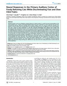
during the entire period of spontaneous activity and acoustic stimulation. This corresponds to typical LNP models computed in previous work (Atencio et al., 2008; Sharpee et al., 2008), Gain, G P[.] = except that we fit the model to the combined response response obtained during acoustic stimulation Background, and spontaneous activity. b Filter output time Second, we considered three LFP-dependent models. The parameters of these models [e.g., G(␪)] were allowed to take four different val1-4Hz Background Gain B C 0.35 ues, one for each binned value of the LFP state 0.3 b G (e.g., delta phase): (1) in the LFP-dependent 0.2 fixed fixed LI 0.3 background (LD-b) model [b(␪), G], the offset 0.1 was allowed to vary with ␪, but the gain was -dep. fixed 0 LD-G fixed; (2) in the LFP-dependent gain (LD-G) 0.25 model [b, G(␪)], gain varied with ␪ but the -dep. fixed background was fixed; and (3) in the LFPLD-b 0.2 dependent gain and background (LD-G&b) model [O(␪), G(␪)], both parameters varied -dep. -dep. LD-G&b 0.15 with ␪. Note that the number of free parame20 0.25 1 4 8 12 16 ters varied across models (for single LFP bands: Frequency [Hz] LI, two parameters; LD-G and LD-b, five parameters; LD-G&b, eight parameters). Finally, as a control condition, we also conD Spontaneous Stimulus sidered an LFP-dependent model without a 60 60 stimulus-driven component (i.e., Eq. 3 with qstim ⫽ 0 at all times). This model only relied on data the variation of background activity to explain 40 40 the data. This model reproduced the observed data very poorly across frequency bands (e.g., 20 20 r 2 ⫽ 0.05 ⫾ 0.01 for delta) and was not analyzed further. 0 We compared the performance of each 0 model in explaining the experimentally obPhase bin served responses using the Akaike information Gain (G) Background (b) 0.8 criterion (AIC), which is a standard model seE 10 lection technique that compensates for the 0.6 variable degrees of freedom between models (Akaike, 1974). The AIC quantifies the descrip0.4 5 tive power of each model based on the loglikelihood of the observed data, penalizing 0.2 models with larger numbers of parameters, and is defined as AIC ⫽ 2 ⫻ k ⫺ 2 ⫻ ln( L), 0 0 where k is the degrees of freedom, and L is the Phase bin log-likelihood of the data under this model. Given that we analyzed multiple repeats of the Figure 2. Response prediction using phase-dependent LNP models. A, Schematic of the LNP model transforming the spectro- stimulus sequence that are unlikely to be statistemporal stimulus representation using a linear filter into a predicted response. The filter activation is passed through an output tically independent, we used an effective denonlinearity characterized by two parameters (G and b) and is used as input for a Poisson spike generator. B, Schematic of the grees of freedom; this was defined as the different models. For additional details, see Materials and Methods. C, Prediction quality (cross-validated) for each model relative number of time bins during the baseline period to the phase of different frequency bands. Inset, Prediction quality relative to the delta band (1– 4 Hz). D, Distribution of spikes plus the number of time bins of one (rather relative to delta phase during stimulus epochs and spontaneous activity for each model (bars) and the actual data (black circles). than all) repeat of the stimulus sequence. We Each bar corresponds to the firing rate in one phase bin. Note that the LI and LD-G models by definition predict the same rate across computed Akaike weights, which quantify the bins. E, Gain and background parameters obtained from each model relative to delta. Each parameter is shown for each phase bin, relative AIC values within a group of models but some models by definition use the same parameter across bins. Error bars denote mean and SEM across units. and which facilitate model comparison within a set of proposed models. For each model, these are defined as exp(⫺0.5 ⫻ AIC) divided by the below) between these models did not provide strong evidence for sum of weights for all models within a group (Burnham and Anderson, either model (0.57 ⫾ 0.07 and 0.42 ⫾ 0.07), and, for simplicity, we 2004). An Akaike weight near 1 suggests a high probability that this restricted our analysis to the nonlinearity described by Equation 2. model minimizes the information lost relative to the actual data comLFP state-dependent models and model comparison. Our goal was to pared with the other models. study how current LFP state (denoted ␪), indexed by the phase or power Note that not all units allow a description based on LNP models. Hence, of a single LFP band or pairs of bands, influenced the stimulus–response we restricted the analysis to those sites for which the LI model reached an r 2 transfer. To this end, we introduced four LNP models that differed in of at least 0.1 (31 of 38 units). Given that we selected sites based on threshold how they include a possible LFP dependency in their model parameters b on performance of the LI model, the better response prediction obtained and G (see Eqs. 2 and 3). All models were fitted using cross-validation to from the LFP-dependent models cannot result from a selection bias. the merged neural responses obtained during stimulus presentation (50 Throughout text, results are presented as mean ⫾ SEM across sites, repeats of the 30 s sequence) and silence (250 s of continuous recording). unless stated otherwise. Statistical comparisons are based on paired t First, we considered an LFP-independent (LI) model, defined by fixed tests, and, when multiple tests are performed between models or gain and background parameters [b, G], i.e., parameters that are constant ii) Linear filter (STRF)

[arb.]

% Spikes / bin

prediction [r2]

×

iii) Output nonlinearity

Spike rate

i) Stimulus representation

Sound frequency

A

iv) Poisson spike train

Kayser et al. • LFP-Dependent Stimulus Encoding in Auditory Cortex

7754 • J. Neurosci., May 20, 2015 • 35(20):7750 –7762

[kHz]

+

20 40

-

Spike rate

0.8 10

Filter output

B

Data

30

LI

LD-G

+

+ o

20

-

LD-b

o

LD-G&b

d

-

10

0

...

...

Trials

I rel(␪) ⫽ 共Itot ⫺ Iignore(␪))/Itot.

Time [ms] -300 +20

A

Firing rate [Spk/s]

frequency bands, these were Bonferroni’s corrected for multiple comparisons. Single-trial stimulus decoding and sensory information. The sensory information carried by the recorded responses and by the responses predicted by the different models was computed using a single-trial decoding approach. For this calculation, we used a nearestneighbor decoder based on the Euclidean distance between the time-binned (10 ms) spike trains observed in individual trials and the trialaveraged spike trains associated with different stimuli, which was shown to work effectively in previous work (Kayser et al., 2010, 2012). As “stimuli” for decoding, we considered 55 sections of 250 ms duration selected within the 30 s stimulus period. From the resulting decoding matrix, we calculated the mutual information between stimuli and responses using established procedures (Quian Quiroga and Panzeri, 2009; Kayser et al., 2010, 2012). To quantify the contribution of spikes during different LFP phases to the mutual information, we repeated the decoding procedure for each unit once by including all spikes (denoted Itot) and then by systematically discarding spikes during each LFP phase ␪ [denoted Iignore(␪)]. From this, we calculated the relative information attributed to spikes during each phase as follows:

The difference between Itot and Iignore(␪) can 1-4Hz be interpreted as the amount of information 500 ms lost when the decoder selectively ignores spikes emitted during a specific phase quadrant, and Figure 3. Example data from LNP models. A, Example data showing the STRFs and nonlinearities for three units. In the STRFs, thus it represents the amount of information red colors indicate time–frequency regions in which increases in acoustic energy drive firing rates and blue regions in which uniquely carried by spikes emitted in the increases in energy reduce firing. The output nonlinearities are shown for the actual data (black) and each model. Note that the gain neglected phase quadrant. Thus, Irel(␪) can (slope) changes for the LD-G model (red), but it remains constant for the LD-b model (green). B, Example data showing the firing be interpreted as the fraction of the total in- rate (trial averaged) for one unit for the actual data (black) and each model during acoustic stimulation. Responses were simulated formation in the spike train that is carried on a single-trial basis. The sound waveform is indicated in the middle, and the bottom displays the delta phase (see example, wave uniquely by spikes emitted at a given phase. for color code) in each trial that was used to shape the SD models. Arrows indicate periods of interest: ⫹, periods in which LFP The normalization by Itot is useful to facilitate phase consistently across trials favors high gain and high background activity, and hence the LD models predict stronger responses comparisons across units carrying different than the LI model; ⫺, periods in which LFP phase consistently favors low gain and background activity, and hence LD models amount of total information. Note that this rel- predict a smaller response than the LI model; o, periods in which the stimulus filter (STRF) predicts no response (hence the LI ative information can be negative and that neg- response is flat) but LFP phase is consistently entrained to the stimulus and hence phase variations in background activity (LD-b, ative values indicate that removing a specific LD-G&b) predict changes in firing rates that coincide with those seen in the actual data; d, periods in which the LFP phase is not set of spikes increases the ability to decode in- systematically aligned with the stimulus and all models predict very similar responses. dividual sensory stimuli. This can happen, for example, when spikes emitted in a given phase silence (spontaneous activity) and during acoustic stimulation are almost completely stimulus unrelated, and thus removing them fawith a series of naturalistic sounds (Fig. 1A). As illustrated by cilitates decoding because it effectively removes noise without removing example data (Fig. 1B), firing rates were modulated systematsignal. We also computed an index of information modulation with ically and reliably by the acoustic stimulus. In addition, inphase, defined as the difference in Irel between the phase bin with highest spection of the LFPs showed that low-frequency network information minus the information in the opposing bin (i.e., 180° apart). To quantify the effect of changes in firing rate with LFP phase on the activity was entrained reliably to the stimulus, as well during modulation of information, we performed the following control analysis. many epochs of the stimulus period (Fig. 1B). This is illustrated in For each unit, we equalized the firing rate across phase bins before stimthe example of Figure 1B by the fact that phase of delta (1– 4 Hz) ulus decoding as follows. We determined the total number of spikes in band is time locked to the stimulus time course reliably across the phase bin across all time points and determined the minimum across trials. This frequent entrainment of slow network activity during bins. Then we randomly removed spikes occurring during the other acoustic stimulation is consistent with previous intracranial rephases to match this minimum number. For each unit, we repeated this process 50 times and averaged the resulting information values. cordings in awake primates and anesthetized rodents (Lakatos et

Results We recorded spiking activity and LFPs from 38 sites in the A1 of six urethane-anesthetized rats using multi-shank silicon tetrodes. Field potentials and spiking responses were recorded both during

al., 2008; Kayser et al., 2009; Szymanski et al., 2011) and neuroimaging results in humans (Howard and Poeppel, 2010; Peelle and Davis, 2012; Ding and Simon, 2013; Gross et al., 2013; Henry et al., 2014). Experimental evidence suggests that fluctuations in slow rhythmic cortical activity reflect changes in network dynam-

Kayser et al. • LFP-Dependent Stimulus Encoding in Auditory Cortex

ics and neural excitability (Bishop, 1933; Azouz and Gray, 1999; Harris and Thiele, 2011; Buzsa´ki et al., 2012; Womelsdorf et al., 2014; Pachitariu et al., 2015; Reig et al., 2015). Hence, the presence of stimulus-locked variations in both firing rates and network activity raises the question of whether and how the sensory encoding of individual neurons depends on the network dynamics captured by LFP activity at different timescales. Firing rates are modulated by LFP phase We first considered the dependence of neuronal firing on the instantaneous phase of individual LFP bands (between 0.25 and 24 Hz). To this end, we partitioned the oscillatory cycle into phase quadrants (i.e., four phase bins; Fig. 1C). Consistent with previous results (Lakatos et al., 2005; Montemurro et al., 2008; Kayser et al., 2009; Haegens et al., 2011), we found that firing rates varied systematically with LFP phase. The degree of firing rate modulation was frequency dependent and was strongest for delta (1– 4 Hz; Fig. 1D) during both acoustic stimulation and spontaneous activity. During acoustic stimulation, the modulation was 44.4 ⫾ 1.2% for delta but only 23.3 ⫾ 0.95% for lower frequencies (0.25– 0.5 Hz), was ⬃15% for alpha (8 –12 Hz) and was ⬍5% for frequencies ⬎20 Hz. During spontaneous activity, similar values were obtained (delta: 49.4 ⫾ 1.9%; ⬍5% for frequencies ⬎20 Hz). The distribution of the preferred phase of firing across units was highly non-uniform for each band during both acoustic stimulation and spontaneous activity (Rayleigh’s test, Z values ⬎ 30 and p ⬍ 10 ⫺11 for all bands). The dependence of firing rates on LFP phase during silence likely reflects an intrinsic modulation of network excitability emerging from local connectivity, cellular properties, or brainwide fluctuations in activity (Schaefer et al., 2006; Harris and Thiele, 2011; Harris and Mrsic-Flogel, 2013; Pachitariu et al., 2015; Reig et al., 2015). The dependence of firing rates on LFP phase during sensory stimulation may either only reflect the same modulation of background firing seen during spontaneous activity but may also reflect an additional dependence of the neuronal stimulus tuning properties on the LFP phase. In the following, we disentangle these contributions using a data-driven modeling approach. LFP state-independent response models To better understand the interaction between the network dynamics indexed by LFP phase and the sensory input, we exploited the possibility to describe A1 responses using receptive fields and LNP models (Depireux et al., 2001; Escabi and Schreiner, 2002; Machens et al., 2004; Rabinowitz et al., 2011; Sharpee et al., 2011). These models provide a quantitative description of both the neural selectivity to the time–frequency content of the sound and their input– output transformation (output nonlinearity; Fig. 2A). To derive such models, we started from a time–frequency representation of the auditory stimulus (Fig. 2Ai) and derived a linear filter (STRFs; Aii) associated with the response of each unit and a static nonlinearity (Aiii) describing the transformation between filter activation and the observed responses. The simulated response was obtained as Poisson spike train obtained from the transformed filter response (Fig. 2Aiv). Traditionally, such models are fit with a fixed set of parameters to the spike trains recorded over the entire period of stimulus presentation. We call this traditional approach the LI model (Fig. 2B). Such a model reflects the best possible (LNP-based) stimulus–response description that ignores the ongoing changes in network activity. Generally, not all units allow a description by STRFs and LNP models (Atencio et al., 2008; Christianson et al.,

J. Neurosci., May 20, 2015 • 35(20):7750 –7762 • 7755

2008). For the present data, 31 of 38 sites allowed a (crossvalidated) response prediction during the stimulus period exceeding a criterion of r 2 ⬎ 0.1. Examples of STRF filters and output nonlinearities are shown in Figure 3A. For subsequent analyses, we modeled these output nonlinearities with a thresholdlinear function (see Eq. 2; quality of fit, r 2 ⫽ 0.96 ⫾ 0.04). The model included also a background parameter b describing additive and not stimulus-related components of the observed response. Thus, the model described the neural responses by specifying its STRF (kept fixed in the following analyses) and two other parameters: (1) the output gain G of the nonlinearity; and (2) the background activity parameter b (Fig. 2Aiii). The gain characterizes the steepness of the output transformation, with higher or lower values reflecting relative amplification or attenuation, respectively. Across units, the average response prediction by the LI model was r 2 ⫽ 0.18 ⫾ 0.01 (Fig. 2C, blue). Although the LI model allowed a reasonable description of the stimulus-driven response, it could not explain the phase dependence of neural firing. This can be seen in Figure 2D, which displays the dependence of firing rates on delta phase. First, during stimulus presentation, the LI model predicts a relatively flat distribution, with only a modest variation across phase bins (4.9 ⫾ 0.5%), which is much weaker than the variation in the actual data (Fig. 2D, left, black circles; 45.0 ⫾ 0.9%; t(30) ⫽ 36; p ⬍ 10 ⫺5). Second, during spontaneous activity, the LI model (by definition) predicts a constant and phase-independent firing rate (Fig. 2D, right), a result that deviates completely from the observed data. Hence, the LI model is insufficient to explain the observed phase dependence of firing rates. LFP state-dependent response models We next considered three extended models in which the model parameters (G, b) could take LFP state-dependent values (Fig. 2B). In the LD-b model, the background firing parameter b varied with LFP state but the gain was fixed. In the LD-G model, the gain was allowed to vary but the background parameter was not. Finally, in the LD-G&b model, both parameters were allowed to vary with LFP state. The results in Figure 2C show that fitting these models relative to LFP phase improved the response prediction considerably. The largest increase in prediction accuracy (r 2) over the LI model occurred for the delta band and reached nearly twice the value obtained with the LI model (0.30 ⫾ 0.02 for the LD-G&b model). Smaller but considerable improvements were observed for lower frequencies (e.g., 0.25– 0.5 Hz) and higher-frequency bands (4 – 8 Hz for theta and 8 –12 Hz for alpha). For frequencies ⬎16 Hz, the improvement in response prediction by LFP-dependent models was small, suggesting that LFP state defined at frequency above 16 Hz does not affect much how cortical neurons encode sounds. Delta phase-dependent response models For the delta band, all LFP-dependent models provided a better response prediction than the LI model. However, the LD-G&b model (r 2 ⫽ 0.30 ⫾ 0.02; Fig. 2C, inset) predicted responses significantly better than the LD-G (r 2 ⫽ 0.24 ⫾ 0.02; t(30) ⫽ 9.7, p ⬍ 10 ⫺5) or LD-b (r 2 ⫽ 0.29 ⫾ 0.02; t(30) ⫽ 4.0, p ⬍ 0.001) model. This result was confirmed by a quantitative model comparison based on Akaike weights, which is less sensitive to differences in the number of model parameters of each model. More than 90% of units had AIC weights larger than 0.95 for the LDG&b model (Akaike weight, 0.96 ⫾ 0.02), providing strong evidence that this model provides the best account of the observed

7756 • J. Neurosci., May 20, 2015 • 35(20):7750 –7762

data within the considered set of models. In addition, the LD-b model also predicted the response significantly better than the LD-G model (t(30) ⫽ 7.3, p ⬍ 10 ⫺5; relative Akaike weights between these models 0.99 ⫾ 0.01 for LD-b), although both had the same number of parameters. Figure 3 illustrates the nature of this improvement in response prediction using example data. Figure 3A illustrates how the LFP dependence affects the output nonlinearity. Figure 3B displays a section of actual data and predicted responses during acoustic stimulation, shown here as trial-averaged firing rates. The bottom of Figure 3B displays the delta phase on each trial used to compute the LD models. This example illustrates the differences between models and the effect on the predicted responses of both the phase values and their reliable entrainment to the sound. The LI model predicts some of the stimulus-induced response peaks but underestimates response amplitudes, predicts temporally more extended peaks than seen in the actual data, and fails to account for rate changes in periods of low firing. When the LFP phase is entrained to the sound (i.e., phase is consistent across trials), the phase variations in gain and background activity increase (Fig. 3A, marked ⫹) or decrease (marked ⫺) the firing rate predicted by the LD models compared with the LI model. When the LFP phase is not entrained (marked “d”), all models predict a firing rate because phase has no consistent effect on LD models. Finally, when LFP phase is stimulus entrained but the linear STRF filter predicts no stimulus response (marked “o”), the phase dependency of background activity still predicts a reliable variation in firing rate (LD-b and LD-G&b) that coincides with firing variations seen in the actual data. In all, this example demonstrates that accurate prediction of the observed responses requires the correct prediction of periods of stimulus drive by the STRF, the LFP-dependent amplification and attenuation of these, and the prediction of responses that are induced by network activity not driven by the stimulus. A similar picture emerged when comparing how different models predicted how firing rate should vary with delta phase (Fig. 2D). The LD-G model predicted some variation of firing rate with phase during stimulation (21.0 ⫾ 0.8%), but these variations were significantly smaller (t(30) ⫽ 31; p ⬍ 10 ⫺5) than those observed in the actual data, which were 45.0 ⫾ 0.9% (Fig. 2D). By definition, this model predicted that firing rates during spontaneous activity do not depend on phase and hence failed to account for the observed state dependence during silence, which was 50.5 ⫾ 1.7%. The LD-b model predicted a firing rate modulation of 43.0 ⫾ 0.4% during stimulation, which was closer to the observed data (t(30) ⫽ 3.5, p ⬍ 0.05) than that of the LD-G model. Moreover, the LD-b model predicted a firing rate modulation during spontaneous activity of 51.9 ⫾ 1.3%, which did not differ significantly from that seen during spontaneous activity (t(30) ⫽ 0.8, p ⬎ 0.05). Finally, the LD-G&b model predicted a firing rate modulation with phase that did not differ from the observed data during both stimulation (45.3 ⫾ 0.4%; t(30) ⫽ 1.5, p ⬎ 0.05) and spontaneous activity (47.2 ⫾ 1.1%; t(30) ⫽ 2.6, p ⬎ 0.05). Phase-dependent sensory gain and background activity To obtain more insights about how the phase dependence of neural responses may affect sensory computations, we report in Figure 2E the distributions of the best-fit values of the gain and background parameters. This leads to a better understanding of how the different models describe the neural responses. For example, the LD-G model necessitates a variation in response gain of a factor of ⬃10 across phase bins, a scale that seems unrealistically large given reported gain modulations in auditory cortical

Kayser et al. • LFP-Dependent Stimulus Encoding in Auditory Cortex

neurons (Rabinowitz et al., 2011; Zhou et al., 2014). In contrast, the LD-G&b model not only provides a better response description but also features more moderate and credible changes in gain of a factor of ⬃2. This lends additional credibility to the LD-G&b model as a better account of the actual data. The distributions of the best-fit gain and background parameters also reveal that both parameters are highest in the first two phase quadrants. These variations in stimulus gain lend themselves to a simple interpretation of how phase dependence affects neural representations: these gain variations implement a relative amplification of sensory inputs during the first half of the delta cycle and an effective attenuation during the second half. Interestingly, gain and background activity vary in a coordinated manner, suggesting that both reflect an overall increase of neural excitability during specific epochs of network dynamics. This dependence of gain and background on LFP phase has direct implications for the information coding properties of auditory neurons, which we explore next. Consequences for sensory information encoding To study the potential effect of state dependence for sensory representations, we quantified the mutual information between neural responses and the stimulus sequence using single-trial decoding. We asked whether the above-described modulation by delta phase of the responses of cortical neurons implies that there are privileged phases of the delta cycle that provide a more important contribution to the total information carried by the entire spike train than other phase epochs. To examine the relative information carried by spikes occurring at different phases of network rhythms, we computed the relative information carried by each phase bin, defined as the difference between the total information provided by the full response (including all spikes from all phases of the delta cycle) and the information carried after removing all spikes occurring during a specific phase bin, normalized by the total information. This quantity can be interpreted as the fraction of the total information in the spike train that is uniquely carried by spikes emitted at a given phase (see Materials and Methods). Large positive values of this quantity indicate that spikes in the considered phase bin carry crucial unique information, whereas negative values indicate that spikes in that bin carry much more noise than stimulus signal and thus removing them facilitates information decoding. We first quantified the relative information for different delta band phase quadrants in the actual data. We found (Fig. 4A) that spikes occurring in the first delta quadrant (the one carrying the most relative information) carried approximately six times more information than spikes emitted during the later quadrant carrying the least relative information (0.34 ⫾ 0.02 vs 0.05 ⫾ 0.01; t(30) ⫽ 9.0, p ⬍ 10 ⫺10; Fig. 4A, black), resulting in an information modulation of 0.29 ⫾ 0.04. Thus, in actual cortical responses, there is a phase-dependent amplification of sensory information at the beginning of the delta cycle compared with later phase epochs. To understand how response gain and background activity contribute to this concentration of information, we computed the information provided by each model and compared it quantitatively with that of the actual data, using the sum of squares across phase quadrants (SS) as measure of the quality of model fit. One factor contributing to the modulation of information with phase may be that the acoustic drive changes on the same timescale. This may happen if network activity becomes entrained to low-frequency variations in the stimulus (Kayser et al., 2009; Schroeder and Lakatos, 2009; Szymanski et al., 2011). Any such contribution is revealed by the LI model, for which any

Kayser et al. • LFP-Dependent Stimulus Encoding in Auditory Cortex

J. Neurosci., May 20, 2015 • 35(20):7750 –7762 • 7757

background activity provided by the model plays a part in shaping informa0.6 0.6 tion content. Finally, we considered the combined 0.4 0.4 effect of phase modulation of both gain and background activity, which is captured by the LD-G&b model. This model 0.2 0.2 yielded information values that were much closer to the actual data (SS, 0.07 ⫾ 0 0 0.01). It predicted them significantly better than the LI (F ⫽ 4.0, p ⬍ 0.01) and all Data LI LD-b LD-G LD-G&b LD (at least F ⫽ 2.1, p ⬍ 0.05) models and -0.2 -0.2 predicted an information modulation Phase bin Phase bin that did not differ significantly from the Figure 4. Phase-dependent sensory information. A, Sensory information carried by spikes in each delta phase quadrant, actual data (0.28 ⫾ 0.02; t(30) ⫽ 0.25, p ⬎ calculated for the actual data (black), and each model. Information is expressed relative to the total information carried by each unit 0.05). Together, these findings demon(Irel; see Materials and Methods). For the actual data, spikes in the first phase quadrant carry the most sensory information strate the following: (1) the phase depencompared with other phase quadrants. B, Sensory information by phase quadrant, after normalizing the number of spikes per dence of gain effectively concentrates phase bin for each unit. Error bars denote mean and SEM across units. sensory information during the early part of the delta cycle; and (2) the phase dependifference in information between phase quadrants can only redence of background activity moderates this concentration of sult from differences in stimulus activation but not changes in information at specific epochs, without preventing it. network dynamics. The higher firing rates in the first quadrant Given that our previous results demonstrated that phase predicted by the LI model (Fig. 2D) suggest a stronger drive durvariations of rate are made of both stimulus-independent and ing the first quadrant, and, indeed, the LI model also predicts stimulus-dependent components, we hypothesized that phase more information for spikes in the first compared with later variations of rate may relate to variations of information in a quadrants (Fig. 4A). However, the LI model failed to describe complex way. In other words, the simultaneous presence of phase accurately the information in the actual data (SS, 0.19 ⫾ 0.03) variations in stimulus gain and background firing suggest that the and resulted in a significantly lower information modulation observed phase dependence of information could not simply be (0.20 ⫾ 0.01; t(30) ⫽ 2.8, p ⬍ 0.01). Hence, phase-dependent explained by the phase dependence of rate. To shed light on this stimulus activation plays a role in shaping the variation in sensory issue, we repeated the information analysis after normalizing information with delta phase but cannot fully explain it, implying spike counts across phase quadrants (Fig. 4B). This revealed that, that phase-dependent variations of cortical activity are required to even when accounting for differences in firing rates, there was a explain the information modulation. considerable residual modulation of information with phase in The effect of the state dependence of output gain on informaboth the actual data (0.19 ⫾ 0.02) and the models (0.19 ⫾ 0.02, tion can be appreciated by comparing the information between 0.61 ⫾ 0.05, 0.15 ⫾ 0.01, and 0.20 ⫾ 0.02 for LI, LD-G, LD-b, and the LI and LD-G models. We expected that adding a stateLD-G&b, respectively). As for the non-normalized information dependent output gain should effectively accentuate the infordata in Figure 4A, we found that also for the normalized data the mation carried by spikes in the first quadrants, because these LD-G&b model provided the closest approximation to the inforreceived the strongest gain (Fig. 2). Indeed, the information valmation of the real cortical responses (SS values for LI, LD-G, ues from the LD-G model peaked in the first quadrant, and the LD-b, and LD-G&b, respectively: 0.17 ⫾ 0.02, 0.25 ⫾ 0.02, information modulation was much larger than for the LI model (0.6 ⫾ 0.06; t(30) ⫽ 22, p ⬍ 10 ⫺10; Fig. 4A), demonstrating that 0.11 ⫾ 0.01, and 0.05 ⫾ 0.005; F tests of LD-G&b vs all others, at phase variations in gain effectively concentrate the sensory inforleast F ⫽ 2.6, p ⬍ 0.05). This shows that increases of firing rates mation during specific epochs of the network cycle. However, the at certain phases cannot be directly interpreted as increases of information modulation of the LD-G model was more extreme information, because phase variations in sensory information than that of actual data, and so this model did not provide a result from phase-dependent changes in stimulus drive comsignificant improvement over the LI model in explaining the acbined with changes in the signal-to-noise ratio of sensory reptual data (SS, 0.14 ⫾ 0.02; F test, F ⫽ 1.9, p ⬎ 0.05), suggesting resentations induced by variations in sensory gain and that other factors need to be included to explain the information background activity. Therefore, to understand how sensory repmodulation in the actual data. resentations are amplified across the cycle cortical state dynamThus, we considered next the effect of background activity on ics, it is necessary to separate variations in stimulus-related sensory information. This is revealed when comparing the LD-b and stimulus-unrelated components of neural activity, as our and SD-G&b models with the LI model. Intuition suggests that models attempt to do. adding the phase-dependent background activity should lead to a We repeated the analysis for other frequency bands and reduction of information in those phase quadrants where this is found that, similar to the modulation of firing rate, the senhighest. Indeed, information values for the LD-b model were sory information was most strongly affected by the phase of highest in the second quadrant, where background activity the delta band. In addition, for all frequency bands, the LDwas weakest (Fig. 2). The LD-b model predicted an informaG&b model provided the best approximation to the observed tion modulation that was comparable with the LI model data, demonstrating that a combination of phase-dependent (0.16 ⫾ 0.01; t(30) ⫽ 1.9, p ⬎ 0.05) but provided a better changes in stimulus-unrelated background activity and senapproximation to the actual data than the LI model (SS, 0.12 ⫾ sory gain are necessary to explain the data. 0.02; F ⫽ 3.4, p ⬍ 0.01), suggesting that the modulation of Rel. information

A

All spikes

B

Normalized spike rates

Kayser et al. • LFP-Dependent Stimulus Encoding in Auditory Cortex

8

5

12 16 20 0.25 1

8 12 16 20 4 Frequency [Hz]

C

0.32

1 4 8

0.18

12

6

Gain (G) 8-12Hz

0.6

4

2

16 20 0.25 1 4 8 12 16 20 Frequency - Background (b)

0.8

[arb.]

4

0.25

[arb.]

Frequency [Hz]

1

B

prediction [r2]

8

Frequency - Gain (G)

A 0.25

Rate modulation [%]

7758 • J. Neurosci., May 20, 2015 • 35(20):7750 –7762

Background (b) 1-4Hz LI LD-G&b

0.4 0.2

0

0 Phase bin

Phase bin

Figure 5. Phase dependence relative to multiple timescales. A, Modulation of firing rates relative to the phase pattern derived from pairs of frequency bands. The color code shows the mean across units of the rate modulation. Note that the resulting values are smaller than for the single-band analysis (Fig. 1) given the higher number of bins (4 ⫻ 4) used here. The strongest modulation is obtained when including the delta band. B, Response prediction provided by the LD-G&b model with gain and background parameters varying independently across frequencies (mean across units). The best response prediction is obtained with b depending on delta phase and G depending on alpha (8 –12 Hz) phase. White circles, Pairs of distinct frequencies for which the LD-G&b model provides a significant (paired t tests, p ⬍ 0.01, Bonferroni’s corrected) improvement in response prediction relative to best-performing single-band model [G(1– 4 Hz); b(1– 4 Hz)]. C, Gain and background parameters of the best-fitting two-band LD-G&b model (red) and the LI model (blue). Error bars denote mean and SEM across units.

Complementary phase dependence exerted by different frequency bands The results presented above were based on models assuming that both stimulus-related (gain G) and unrelated (background b) contributions depend on the LFP phase at the same frequency. However, it could in principle be that stimulus–response gain and background firing relate to distinct timescales of network activity. Indeed, prominent theories have suggested that different rhythms exert a differential control on stimulus processing (Lisman, 2005; Panzeri et al., 2010; Jensen et al., 2012, 2014; Bastos et al., 2015), such as the multiplexing of sensory representations and their temporal segmentation in theta and gamma band activity (Lisman, 2005) or the relative contribution of gamma and beta rhythms to feedforward and feedback transmission (Bastos et al., 2015). To test whether this was the case here, we extended the above analysis by now allowing parameters G and b of the LDG&b model to each dependent on distinct frequency band. First, we analyzed the phase dependence of firing rates relative to all pairs of frequency bands. This revealed that the firing rate modulation was strongest computed relative to pairs of bands involving the delta band and frequencies between 2 and 12 Hz (Fig. 5A). This suggests that including the LFP dependence relative to multiple bands may indeed improve the predictive power of stimulus–response models. Then we repeated the model optimization by varying G and b with the phase of independent bands. This revealed (Fig. 5B) a strong dependence of response prediction on the band used to optimize the background parameter b, with best predictions occurring when b was dependent on delta. Varying the band for gain also affected response prediction, although to a smaller degree. The best-fitting two-band LD-G&b model was found for the combination of b(1– 4 Hz) and G(8 –12 Hz) and provided a predictive power of r 2 ⫽ 0.33 ⫾ 0.02. To determine whether this two-band model indeed provides a significant predictive benefit compared with any single-band model, we compared the prediction of all two-band models to the best-performing single-band model [i.e., G(1– 4 Hz); b(1– 4 Hz)]. The prediction performance was improved significantly (paired t tests, Bonferroni’s corrected, p ⬍ 0.01) for the combinations of b(1– 4 Hz) with G(2– 6, 4 – 8, 8 –12, 10 –14 Hz). To determine which combinations of frequency bands and models provide the best response prediction of all models considered, we compared the Akaike weights across all combinations of models and pairs of frequency bands (4 ⫻ 169 combinations). This revealed that the most likely model was the

combination [b(1– 4 Hz), G(8 –12 Hz)], with an average Akaike weight of 0.31 ⫾ 0.08. Models not based on background activity derived from delta or using a response gain based on frequencies outside the range of 2–12 Hz had Akaike weights ⬍10 ⫺5. This suggests that phase variations in stimulus-unrelated firing and stimulus–response gain relate to distinct timescales of network activity, with variations in background activity being related specifically to the delta band and higher frequencies between 2 and 12 Hz reflecting changes in sensory gain. The parameters of the best two-band model are shown in Figure 5C. These confirm the above result that LFP-dependent models result in rhythmic variations in stimulus-unrelated firing and sensory gain, which (as seen above) result in a concentration of sensory information during parts of the network cycle. Cortical states and phase-dependent coding Previous work has shown that neural response properties and the patterns of sensory encoding change with the general state of cortical activity (Curto et al., 2009; Harris and Thiele, 2011; Marguet and Harris, 2011; Ecker et al., 2014; Pachitariu et al., 2015). Usually the state of cortical activity is inferred from the ratio between power of low-frequency rhythmic activity (⬍10 Hz) and total power and/or from the pattern of correlations between neurons. Prominent low-frequency activity is a sign of a synchronized state in which many neurons respond in a coordinated manner (Marguet and Harris, 2011; Sakata and Harris, 2012; Pachitariu et al., 2015). Based on the assessment of the ratio of low-frequency LFP power to the total LFP power, we found that cortical state was mostly stable during our recordings and tended toward the synchronized state (Fig. 6A). Only one of six experiments revealed stronger transitions in low-frequency activity over the time course of the recordings (Fig. 6A, black). However, inspection of LD models separately for each experiment showed that the same main result presented in Figure 5B was observed consistently across individual experiments and holds regardless of minor changes in cortical state (Fig. 6B). State dependence relative to the power of network rhythms Given that previous studies have shown that firing rates can be related to the power of LFP bands across a range of frequency bands (Lakatos et al., 2005; Kayser et al., 2009; Haegens et al., 2011), we completed our study by repeating the above analysis using the power rather than the phase of individual LFP bands. This effectively quantifies to which degree changes in LFP power

Kayser et al. • LFP-Dependent Stimulus Encoding in Auditory Cortex

LFP power ratio

A

J. Neurosci., May 20, 2015 • 35(20):7750 –7762 • 7759

1 0.8 0.6 0.4 0.2 Spontaneous 0 0 250 0

Frequency - Gain (G)

B

Stimulus 250

500 750 Time [s]

1000 1250 1500

[r2] 0.10

0.22

0.20

0.34

0.16

0.34

0.25 4 12 20 0.25 4 12 20 Frequency - Background (b)

Figure 6. Consistency of results across experiments and variations in cortical state. A, To characterize the stability of cortical state during recordings, we quantified the ratio of lowfrequency LFP power (0.25–5 Hz) to the total LFP power (0.25–50 Hz). This is shown here for three example experiments (averaged across all recording channels). For two of these, the cortical state was stable both during spontaneous activity and sensory stimulation, whereas one experiment (black) exhibited larger fluctuations in power ratio during the stimulus presentation period. B, Average response prediction provided by two-band LD-G&b models (compare with Fig. 5B) for each of the three experiments shown in A. The similar pattern of results was observed consistently across all experiments.

within a stable cortical state relate to changes in firing rates and LFP-dependent patterns of sensory encoding. To this end, we divided the range of power values observed on each LFP channel into four equally populated bins. We found that a modulation of firing rate with LFP power was evident for all frequencies tested (Fig. 7A). In general, firing rates were highest when the LFP power was strongest. We then asked whether including power dependency into the LNP models would provide a similar benefit in response prediction as found for phase. An increase in predictive power relative to the LI model was evident for all LD models for frequency bands ⬎1 Hz. However, similar to the firing rate modulation, the predictive power varied little with LFP band (Fig. 7B). In addition, the overall increase in response prediction was smaller for LFP power than for LFP phase. For example, the best performing single-band model for power [LD-b(8 –12 Hz)] improved response prediction by less than half the amount as obtained by the best single-band model for phase [LD-G&b(1– 4 Hz)]. Importantly, for none of the frequency bands tested did the predictive power of the LD-G&b model excel beyond that of the LD-b model (paired t tests, p ⬎ 0.05). This suggests that the improvement in response prediction by including state dependence relative to LFP power is primarily explained by changes in stimulus-unrelated background activity and does not relate to changes in sensory gain.

Discussion We found that response models for A1 neurons yield higher predictive power when including variations in sensory gain and stimulus-unrelated activity relative to the timing (phase) of rhythmic network activity. In particular, we found that changes in stimulus-unrelated firing relate to delta phase, whereas changes in sensory gain relate to the phase of frequency bands between 2

and 12 Hz. Our results show that stimulus–response transformations can only be understood when placed in the context of ongoing network dynamics and provide a modeling framework to understand such LFP-dependent responses. Second, they suggest a differential effect of auditory cortical network activity at different timescales on sound encoding. Third, they suggest a neural mechanism by which network rhythms may implement the rhythmic amplification of sound tokens and the rhythmic concentration of sensory information, a prominent hypothesis put forward previously. The role of network rhythms for auditory perception Natural sounds are highly structured at timescales below ⬃12 Hz, and this structure is of critical importance for perception (Rosen, 1992; Ghitza and Greenberg, 2009). Combined with the prominence of rhythmic activity in the A1 at similar scales (Schroeder and Lakatos, 2009; Ding and Simon, 2013; Doelling et al., 2014; Gross et al., 2013), this has led to the hypothesis that the A1 rhythmically samples the environment at these specific timescales (Giraud and Poeppel, 2012; Zion Golumbic et al., 2012; Leong and Goswami, 2014). Support for this hypothesis comes from studies showing that the firing rate of auditory neurons varies with LFP phase (Lakatos et al., 2005; Kayser et al., 2009) and from neuroimaging studies showing that slow cortical rhythms align to acoustic landmarks (Doelling et al., 2014; Gross et al., 2013; Arnal et al., 2014) and are predictive of sound detection or intelligibility (Ng et al., 2012; Peelle and Davis, 2012; Ding and Simon, 2013; Henry et al., 2014; Strauß et al., 2015). However, previous studies did not provide a functional description of the neural computations that may link network rhythms to changes in sound encoding (Giraud and Poeppel, 2012; Poeppel, 2014). Our results fill this gap and provide a model-driven understanding of how different network rhythms shape sound encoding. First, we found that LI models cannot account for the observed phase dependence of responses. Hence, the correlated stimulus drive to both network rhythms and individual neurons is not sufficient to explain phase-dependent firing rates. Second, we found that purely stimulus-unrelated variations in background activity are also insufficient to explain this phase dependence. Rather, an LFP-dependent output gain is necessary for a more accurate response prediction. Third, our information theoretic analysis shows that a phase-dependent sensory gain effectively leads to an attenuation of sensory inputs during specific epochs of the network cycle and thereby concentrates sensory information in time. This demonstrates that the phase dependence of A1 responses, at least in part, relates to a direct rhythmic modulation of neural sound encoding. Our results support the hypothesis that the alignment of rhythmic auditory cortical activity to acoustic landmarks helps to selectively amplify those sound tokens that are aligned with the most excitable phase of the network (Schroeder and Lakatos, 2009; Giraud and Poeppel, 2012; Lakatos et al., 2013). Previous work demonstrated a correlation between network dynamics and firing rates, yet this does not necessarily imply a phase dependence of sensory information; any modulation of firing rates could simply result from changes in stimulus-unrelated activity. However, our modeling approach allows disentangling these contributions and shows that LFP phase relates to systematic changes in stimulus– response gain. Hence, LFP-dependent transformations in A1 can indeed serve to selectively amplify the encoding of appropriate timed sound tokens (Lakatos et al., 2013; Arnal et al., 2014).

Kayser et al. • LFP-Dependent Stimulus Encoding in Auditory Cortex

7760 • J. Neurosci., May 20, 2015 • 35(20):7750 –7762

A

Stimulus

% Rate Modulation 30 60

Spontaneous 0

B 0.3

1

prediction [r2]

Frequency [Hz]

0.25 4 8 12 16 20

50 Low High 10 Power bin % Spikes/bin

LI

LD-G

LD-b LD-G&b

0.25 0.2 0.15 0.25

1

4

8

12

16

20

Frequency [Hz]

Figure 7. Response dependence relative to the power of LFP bands. A, Distribution of firing rates across LFP power bins for different bands during acoustic stimulation and spontaneous activity. Color codes are the average across units. Right, Modulation of firing rate. B, Response prediction derived from LFP-dependent models rendering gain and/or background dependent on the power of LFP bands. Error bars denote mean and SEM across units.

Multiple rhythms shape neural responses in the A1 Previous studies highlighted the importance of rhythmic activity at multiple timescales for hearing. For example, delta band activity has been linked to temporal prediction (Schroeder and Lakatos, 2009; Stefanics et al., 2010; Arnal et al., 2014), whereas activity in the theta and alpha bands has been linked to sound detection (Ng et al., 2012; Peelle and Davis, 2012; Leske et al., 2013; Henry et al., 2014) and stream selection (Zion Golumbic et al., 2013; Strauß et al., 2014b). In line with this, we found that A1 responses are modulated by the phase and power of network activity at various timescales, prominently including the delta band and frequencies around the theta and alpha bands. Importantly, our results differentiate the role of delta and higher frequencies and relate these with changes in stimulus-unrelated spiking and output gain, respectively. This concords with a previous hypothesis about activity in the theta and alpha bands being critical for the prediction of upcoming sound structure (Ghitza and Greenberg, 2009; Ghitza, 2011; Peelle and Davis, 2012) or the gating of auditory perception by task demands (Strauß et al., 2014a; Wilsch et al., 2014). State-dependent coding as a general feature of cortical computation Previous work revealed task-related changes in auditory receptive fields (Fritz et al., 2007) and suggested that changes in the output nonlinearity (Escabi and Schreiner, 2002; Ahrens et al., 2008) or synaptic timescales (David and Shamma, 2013) may be underlying these. Our results show that such changes in sound encoding may be tightly linked to the network dynamics as reflected by LFPs. More generally, our results foster the general notion of statedependent computations in cortical circuits (Curto et al., 2009; Harris and Thiele, 2011; Sharpee et al., 2011; Womelsdorf et al., 2014). Previous studies have shown that patterns of population activity are highly structured relative to signatures of network state, such as slow rhythms or population spikes (Lisman, 2005; Sakata and Harris, 2009; Luczak et al., 2013), and showed that knowledge about the current network state can account for a large fraction of response variance and pairwise neural correlations (Curto et al., 2009; Ecker et al., 2014; Goris et al., 2014). Like many recent studies on the encoding of complex sounds (Escabi and Schreiner, 2002; Ahrens et al., 2008; Curto et al., 2009; Rabinowitz et al., 2011), the present data were obtained under anesthesia. We found that the cortical state during our recordings, as indexed by low-frequency LFP power, was mostly stable. Hence, our results reflect the effect of changes in faster network dynamics

reflected by the LFP phase ⬎1 Hz on sound encoding. Complementary to this, previous work has shown that transitions from desynchronized to synchronized cortical states result in the loss of temporal spike precision, a dramatic reduction of sensory coding fidelity, and an increase in noise correlations between neurons (Marguet and Harris, 2011; Pachitariu et al., 2015). Hence, our results extend previous insights on state-dependent coding and demonstrate that the amount of encoded sensory information is modulated by both slowly changing cortical states and the network dynamics at faster timescales. Interestingly, recent studies demonstrated that state transitions may result in a change in synaptic gain, a possible mechanism that could also explain the phase dependence of sensory gain observed here (Reig et al., 2015), and revealed that firing patterns during synchronized states can be partly explained by taking into account knowledge about the state of recurrent network excitation (Curto et al., 2009), which is possibly related to the systematic and correlated changes in sensory gain and background activity observed here. The key signatures of phase-dependent sensory encoding are observed in both humans and animals (Giraud and Poeppel, 2012; Ng et al., 2013; Jensen et al., 2014). Although the direct influence of phasedependent sensory gain or background activity on perception remains to be studied, previous evidence from monkeys (Lakatos et al., 2013) and humans (Ng et al., 2012; Henry et al., 2014; Strauß et al., 2015) strongly suggests that phase-dependent sound encoding indeed has an influence on human perception. Implications for hearing Our results reveal that phase-dependent neural computations lead to an effective concentration of sensory information within specific epochs of the network cycle. This chunking of acoustic information may have key implications for perception. First, it could help to prioritize the processing of novel events by emphasizing initial transients and thereby could help to segment individual sound tokens in time. Such a role of network rhythms in parsing sensory inputs has been proposed similarly in vision (Jensen et al., 2014). Second, it may facilitate the selective transmission of information by temporally multiplexed coding schemes. These generally require a rhythmic modulation of response gain to facilitate the readout of individual messages from a multiplexed response (Panzeri et al., 2010; Akam and Kullmann, 2014). Furthermore, our results suggest that frequencies including the alpha band may be linked to sensory gain. Previously, reduced auditory cortical alpha activity has been linked to tinnitus (Weisz et al., 2005; Leske et al., 2013), with the interpretation that deviations from the normal state of alpha activity allows local populations to

Kayser et al. • LFP-Dependent Stimulus Encoding in Auditory Cortex

engage in abnormal sensory representations (Eggermont and Roberts, 2004; Weisz et al., 2011). Such abnormal sensory representations may, for example, result from a reduced control over sensory gain by network mechanisms such as those reported here.

References Ahrens MB, Linden JF, Sahani M (2008) Nonlinearities and contextual influences in auditory cortical responses modeled with multilinear spectrotemporal methods. J Neurosci 28:1929 –1942. CrossRef Medline Akaike H (1974) A new look at the statistical model identification. IEEE Trans Automat Contr 19:716 –723. CrossRef Akam T, Kullmann DM (2014) Oscillatory multiplexing of population codes for selective communication in the mammalian brain. Nat Rev Neurosci 15:111–122. CrossRef Medline Arnal LH, Doelling KB, Poeppel D (2014) Delta-beta coupled oscillations underlie temporal prediction accuracy. Cereb Cortex. Advance online publication. Retrieved March 12, 2015. doi:10.1093/cercor/bhu103. CrossRef Medline Atencio CA, Sharpee TO, Schreiner CE (2008) Cooperative nonlinearities in auditory cortical neurons. Neuron 58:956 –966. CrossRef Medline Azouz R, Gray CM (1999) Cellular mechanisms contributing to response variability of cortical neurons in vivo. J Neurosci 19:2209 –2223. Medline Bastos AM, Vezoli J, Bosman CA, Schoffelen JM, Oostenveld R, Dowdall JR, De Weerd P, Kennedy H, Fries P (2015) Visual areas exert feedforward and feedback influences through distinct frequency channels. Neuron 85:390 – 401. CrossRef Medline Belitski A, Gretton A, Magri C, Murayama Y, Montemurro MA, Logothetis NK, Panzeri S (2008) Low-frequency local field potentials and spikes in primary visual cortex convey independent visual information. J Neurosci 28:5696 –5709. CrossRef Medline Bishop G (1933) Cyclic changes in the excitability of the optic pathway of the rabbit. Am J Physiol 103:213–224. Burnham KP, Anderson DR (2004) Multimodel inference: understanding AIC and BIC in model selection. Sociol Methods Res 33:261–304. CrossRef Buzsa´ki G, Anastassiou CA, Koch C (2012) The origin of extracellular fields and currents—EEG, ECoG, LFP and spikes. Nat Rev Neurosci 13:407– 420. CrossRef Medline Canolty RT, Knight RT (2010) The functional role of cross-frequency coupling. Trends Cogn Sci 14:506 –515. CrossRef Medline Christianson GB, Sahani M, Linden JF (2008) The consequences of response nonlinearities for interpretation of spectrotemporal receptive fields. J Neurosci 28:446 – 455. CrossRef Medline Curto C, Sakata S, Marguet S, Itskov V, Harris KD (2009) A simple model of cortical dynamics explains variability and state dependence of sensory responses in urethane-anesthetized auditory cortex. J Neurosci 29: 10600 –10612. CrossRef Medline David SV, Shamma SA (2013) Integration over multiple timescales in primary auditory cortex. J Neurosci 33:19154 –19166. CrossRef Medline David SV, Mesgarani N, Shamma SA (2007) Estimating sparse spectrotemporal receptive fields with natural stimuli. Network 18:191–212. CrossRef Medline Depireux DA, Simon JZ, Klein DJ, Shamma SA (2001) Spectro-temporal response field characterization with dynamic ripples in ferret primary auditory cortex. J Neurophysiol 85:1220 –1234. Medline Ding N, Simon JZ (2012) Neural coding of continuous speech in auditory cortex during monaural and dichotic listening. J Neurophysiol 107: 78 – 89. CrossRef Medline Ding N, Simon JZ (2013) Adaptive temporal encoding leads to a backgroundinsensitive cortical representation of speech. J Neurosci 33:5728 –5735. CrossRef Medline Doelling KB, Arnal LH, Ghitza O, Poeppel D (2014) Acoustic landmarks drive delta-theta oscillations to enable speech comprehension by facilitating perceptual parsing. Neuroimage 85:761–768. CrossRef Medline Ecker AS, Berens P, Cotton RJ, Subramaniyan M, Denfield GH, Cadwell CR, Smirnakis SM, Bethge M, Tolias AS (2014) State dependence of noise correlations in macaque primary visual cortex. Neuron 82:235–248. CrossRef Medline Eggermont JJ, Roberts LE (2004) The neuroscience of tinnitus. Trends Neurosci 27:676 – 682. CrossRef Medline Escabi MA, Schreiner CE (2002) Nonlinear spectrotemporal sound analysis by neurons in the auditory midbrain. J Neurosci 22:4114 – 4131. Medline

J. Neurosci., May 20, 2015 • 35(20):7750 –7762 • 7761 Fritz JB, Elhilali M, Shamma SA (2007) Adaptive changes in cortical receptive fields induced by attention to complex sounds. J Neurophysiol 98: 2337–2346. CrossRef Medline Ghitza O (2011) Linking speech perception and neurophysiology: speech decoding guided by cascaded oscillators locked to the input rhythm. Front Psychol 2:130. Medline Ghitza O, Greenberg S (2009) On the possible role of brain rhythms in speech perception: intelligibility of time-compressed speech with periodic and aperiodic insertions of silence. Phonetica 66:113–126. CrossRef Medline Giraud AL, Poeppel D (2012) Cortical oscillations and speech processing: emerging computational principles and operations. Nat Neurosci 15: 511–517. CrossRef Medline Goris RL, Movshon JA, Simoncelli EP (2014) Partitioning neuronal variability. Nat Neurosci 17:858 – 865. CrossRef Medline Gross J, Hoogenboom N, Thut G, Schyns P, Panzeri S, Belin P, Garrod S (2013) Speech rhythms and multiplexed oscillatory sensory coding in the human brain. PLoS Biol 11:e1001752. CrossRef Medline Haegens S, Na´cher V, Luna R, Romo R, Jensen O (2011) alpha-Oscillations in the monkey sensorimotor network influence discrimination performance by rhythmical inhibition of neuronal spiking. Proc Natl Acad Sci U S A 108:19377–19382. CrossRef Medline Harris KD, Mrsic-Flogel TD (2013) Cortical connectivity and sensory coding. Nature 503:51–58. CrossRef Medline Harris KD, Thiele A (2011) Cortical state and attention. Nat Rev Neurosci 12:509 –523. CrossRef Medline Hazan L, Zugaro M, Buzsa´ki G (2006) Klusters, NeuroScope, NDManager: a free software suite for neurophysiological data processing and visualization. J Neurosci Methods 155:207–216. CrossRef Medline Henry MJ, Herrmann B, Obleser J (2014) Entrained neural oscillations in multiple frequency bands comodulate behavior. Proc Natl Acad Sci U S A 111:14935–14940. CrossRef Medline Howard MF, Poeppel D (2010) Discrimination of speech stimuli based on neuronal response phase patterns depends on acoustics but not comprehension. J Neurophysiol 104:2500 –2511. CrossRef Medline Jensen O, Bonnefond M, VanRullen R (2012) An oscillatory mechanism for prioritizing salient unattended stimuli. Trends Cogn Sci 16:200 –206. CrossRef Medline Jensen O, Gips B, Bergmann TO, Bonnefond M (2014) Temporal coding organized by coupled alpha and gamma oscillations prioritize visual processing. Trends Neurosci 37:357–369. CrossRef Medline Kayser C (2009) Phase resetting as a mechanism for supramodal attentional control. Neuron 64:300 –302. CrossRef Medline Kayser C, Montemurro MA, Logothetis NK, Panzeri S (2009) Spike-phase coding boosts and stabilizes information carried by spatial and temporal spike patterns. Neuron 61:597– 608. CrossRef Medline Kayser C, Logothetis NK, Panzeri S (2010) Millisecond encoding precision of auditory cortex neurons. Proc Natl Acad Sci U S A 107:16976 –16981. CrossRef Medline Kayser C, Ince RA, Panzeri S (2012) Analysis of slow (theta) oscillations as a potential temporal reference frame for information coding in sensory cortices. PLoS Comput Biol 8:e1002717. CrossRef Medline Lakatos P, Shah AS, Knuth KH, Ulbert I, Karmos G, Schroeder CE (2005) An oscillatory hierarchy controlling neuronal excitability and stimulus processing in the auditory cortex. J Neurophysiol 94:1904 –1911. CrossRef Medline Lakatos P, Karmos G, Mehta AD, Ulbert I, Schroeder CE (2008) Entrainment of neuronal oscillations as a mechanism of attentional selection. Science 320:110 –113. CrossRef Medline Lakatos P, Musacchia G, O’Connel MN, Falchier AY, Javitt DC, Schroeder CE (2013) The spectrotemporal filter mechanism of auditory selective attention. Neuron 77:750 –761. CrossRef Medline Leong V, Goswami U (2014) Assessment of rhythmic entrainment at multiple timescales in dyslexia: evidence for disruption to syllable timing. Hear Res 308:141–161. CrossRef Medline Leske S, Tse A, Oosterhof NN, Hartmann T, Mu¨ller N, Keil J, Weisz N (2013) The strength of alpha and beta oscillations parametrically scale with the strength of an illusory auditory percept. Neuroimage 88C:69 –78. CrossRef Medline Lisman J (2005) The theta/gamma discrete phase code occuring during the hippocampal phase precession may be a more general brain coding scheme. Hippocampus 15:913–922. CrossRef Medline

7762 • J. Neurosci., May 20, 2015 • 35(20):7750 –7762 Luczak A, Bartho P, Harris KD (2013) Gating of sensory input by spontaneous cortical activity. J Neurosci 33:1684 –1695. CrossRef Medline Machens CK, Wehr MS, Zador AM (2004) Linearity of cortical receptive fields measured with natural sounds. J Neurosci 24:1089 –1100. CrossRef Medline Marguet SL, Harris KD (2011) State-dependent representation of amplitudemodulated noise stimuli in rat auditory cortex. J Neurosci 31:6414 – 6420. CrossRef Medline Mesgarani N, Chang EF (2012) Selective cortical representation of attended speaker in multi-talker speech perception. Nature 485:233–236. CrossRef Medline Montemurro MA, Rasch MJ, Murayama Y, Logothetis NK, Panzeri S (2008) Phase-of-firing coding of natural visual stimuli in primary visual cortex. Curr Biol 18:375–380. CrossRef Medline Ng BSW, Logothetis NK, Kayser C (2013) EEG phase patterns reflect the selectivity of neural firing. Cereb Cortex 23:389 –398. CrossRef Medline Ng BS, Schroeder T, Kayser C (2012) A precluding but not ensuring role of entrained low-frequency oscillations for auditory perception. J Neurosci 32:12268 –12276. CrossRef Medline Pachitariu M, Lyamzin DR, Sahani M, Lesica NA (2015) State-dependent population coding in primary auditory cortex. J Neurosci 35:2058 –2073. CrossRef Medline Panzeri S, Brunel N, Logothetis NK, Kayser C (2010) Sensory neural codes using multiplexed temporal scales. Trends Neurosci 33:111–120. CrossRef Medline Peelle JE, Davis MH (2012) Neural oscillations carry speech rhythm through to comprehension. Front Psychol 3:320. CrossRef Medline Peelle JE, Gross J, Davis MH (2013) Phase-locked responses to speech in human auditory cortex are enhanced during comprehension. Cereb Cortex 23:1378 –1387. CrossRef Medline Poeppel D (2014) The neuroanatomic and neurophysiological infrastructure for speech and language. Curr Opin Neurobiol 28:142–149. CrossRef Medline Quian Quiroga R, Panzeri S (2009) Extracting information from neuronal populations: information theory and decoding approaches. Nat Rev Neurosci 10:173–185. CrossRef Medline Rabinowitz NC, Willmore BD, Schnupp JW, King AJ (2011) Contrast gain control in auditory cortex. Neuron 70:1178 –1191. CrossRef Medline Reig R, Zerlaut Y, Vergara R, Destexhe A, Sanchez-Vives MV (2015) Gain modulation of synaptic inputs by network state in auditory cortex in vivo. J Neurosci 35:2689 –2702. CrossRef Medline Rosen S (1992) Temporal information in speech: acoustic, auditory and linguistic aspects. Philos Trans R Soc Lond B Biol Sci 336:367–373. CrossRef Medline Sakata S, Harris KD (2009) Laminar structure of spontaneous and sensoryevoked population activity in auditory cortex. Neuron 64:404 – 418. CrossRef Medline Sakata S, Harris KD (2012) Laminar-dependent effects of cortical state on auditory cortical spontaneous activity. Front Neural Circuits 6:109. CrossRef Medline Schaefer AT, Angelo K, Spors H, Margrie TW (2006) Neuronal oscillations enhance stimulus discrimination by ensuring action potential precision. PLoS Biol 4:e163. CrossRef Medline Schmitzer-Torbert N, Jackson J, Henze D, Harris K, Redish AD (2005) Quantitative measures of cluster quality for use in extracellular recordings. Neuroscience 131:1–11. CrossRef Medline Schroeder CE, Lakatos P (2009) Low-frequency neuronal oscillations as in-

Kayser et al. • LFP-Dependent Stimulus Encoding in Auditory Cortex struments of sensory selection. Trends Neurosci 32:9 –18. CrossRef Medline Sharpee TO, Miller KD, Stryker MP (2008) On the importance of static nonlinearity in estimating spatiotemporal neural filters with natural stimuli. J Neurophysiol 99:2496 –2509. CrossRef Medline Sharpee TO, Atencio CA, Schreiner CE (2011) Hierarchical representations in the auditory cortex. Curr Opin Neurobiol 21:761–767. CrossRef Medline Stefanics G, Hangya B, Herna´di I, Winkler I, Lakatos P, Ulbert I (2010) Phase entrainment of human delta oscillations can mediate the effects of expectation on reaction speed. J Neurosci 30:13578 –13585. CrossRef Medline Strauß A, Wo¨stmann M, Obleser J (2014a) Cortical alpha oscillations as a tool for auditory selective inhibition. Front Hum Neurosci 8:350. CrossRef Medline Strauß A, Kotz SA, Scharinger M, Obleser J (2014b) Alpha and theta brain oscillations index dissociable processes in spoken word recognition. Neuroimage 97:387–395. CrossRef Medline Strauß A, Henry MJ, Scharinger M, Obleser J (2015) Alpha phase determines successful lexical decision in noise. J Neurosci 35:3256 –3262. CrossRef Medline Szymanski FD, Rabinowitz NC, Magri C, Panzeri S, Schnupp JW (2011) The laminar and temporal structure of stimulus information in the phase of field potentials of auditory cortex. J Neurosci 31:15787–15801. CrossRef Medline Takekawa T, Isomura Y, Fukai T (2010) Accurate spike sorting for multiunit recordings. Eur J Neurosci 31:263–272. CrossRef Medline Theunissen FE, David SV, Singh NC, Hsu A, Vinje WE, Gallant JL (2001) Estimating spatio-temporal receptive fields of auditory and visual neurons from their responses to natural stimuli. Network 12:289 –316. CrossRef Medline Vanrullen R, Busch NA, Drewes J, Dubois J (2011) Ongoing EEG phase as a trial-by-trial predictor of perceptual and attentional variability. Front Psychol 2:60. CrossRef Medline Weisz N, Moratti S, Meinzer M, Dohrmann K, Elbert T (2005) Tinnitus perception and distress is related to abnormal spontaneous brain activity as measured by magnetoencephalography. PLoS Med 2:e153. CrossRef Medline Weisz N, Hartmann T, Mu¨ller N, Lorenz I, Obleser J (2011) Alpha rhythms in audition: cognitive and clinical perspectives. Front Psychol 2:73. CrossRef Medline Wilsch A, Henry MJ, Herrmann B, Maess B, Obleser J (2014) Alpha oscillatory dynamics index temporal expectation benefits in working memory. Cereb Cortex. Advance online publication. Retrieved April 12, 2015. doi: 10.1093/cercor/bhu004. CrossRef Medline Womelsdorf T, Valiante TA, Sahin NT, Miller KJ, Tiesinga P (2014) Dynamic circuit motifs underlying rhythmic gain control, gating and integration. Nat Neurosci 17:1031–1039. CrossRef Medline Zhou M, Liang F, Xiong XR, Li L, Li H, Xiao Z, Tao HW, Zhang LI (2014) Scaling down of balanced excitation and inhibition by active behavioral states in auditory cortex. Nat Neurosci 17:841– 850. CrossRef Medline Zion Golumbic EM, Poeppel D, Schroeder CE (2012) Temporal context in speech processing and attentional stream selection: a behavioral and neural perspective. Brain Lang 122:151–161. CrossRef Medline Zion Golumbic EM, Ding N, Bickel S, Lakatos P, Schevon CA, McKhann GM, Goodman RR, Emerson R, Mehta AD, Simon JZ, Poeppel D, Schroeder CE (2013) Mechanisms underlying selective neuronal tracking of attended speech at a “cocktail party.” Neuron 77:980 –991. CrossRef