Rotor speed estimation for indirect stator flux oriented induction motor ...

Youssef Agrebi

J. Electrical Systems 3-3 (2007): 131-143

Moncef Triki

Regular paper

Yassine Koubaa Mohamed Boussak

Rotor speed estimation for indirect stator flux oriented induction motor drive based on MRAS scheme

JES Journal of Electrical Systems

In this paper, a conventional indirect stator flux oriented controlled (ISFOC) induction motor drive is presented. In order to eliminate the speed sensor, an adaptation algorithm for tuning the rotor speed is proposed. Based on the model reference adaptive system (MRAS) scheme, the rotor speed is tuned to obtain an exact ISFOC induction motor drive. The reference and adjustable models, developed in stationary stator reference frame, are used in the MRAS scheme to estimate induction rotor peed from measured terminal voltages and currents. The IP gains speed controller and PI gains current controller are calculated and tuned at each sampling time according to the new estimated rotor speed. The proposed algorithm has been tested by numerical simulation, showing the capability of driving active load; and stability is preserved. Experimental results obtained with a general-purpose 1-kW induction machine are presented showing the effectiveness of the proposed approach in terms of dynamic performance. Keywords: indirect stator field orientation, induction motor drive, model reference adaptive

system (MRAS), rotor speed estimation 1. INTRODUCTION The AC induction motor has been gradually replacing the DC motor in many applications due to its reliability, ruggedness and relatively low cost. Unfortunately, they have nonlinear dynamics and, for variable speed servo applications, they require advanced control schemes. Fortunately, however, using power electronics and fast digital signal processors (DSP), the implementation of such advanced controllers is now becoming practical [5]. For high-performance vector-controlled induction motor (IM) drives, speed information is necessary. This information is generally provided by a sensor, such as a resolver or an encoder. Due to the cost and fragility of mechanical speed sensors and to the difficulty of installing that kind of sensor in many applications, speed-sensorless systems, in which rotor speed measurements are not available, are preferred and find applications in many areas such as robotics manipulators, mechanical tool drives, and other industrial fields [12]. A several schemes have been proposed for speed-sensorless vector-controlled induction motor (IM) drives, which implies the estimation of the mechanical speed from the only measurements of the stator currents and voltages. The advantages of sensorless drives are clear: the mechanical setup and maintenance are less troublesome, and the reliability, especially in hostile environments, is improved if the mechanical transducer is removed. Among the various approaches that have been proposed, the observer-based [2],[6]–[10] and the model-reference-adaptive-system (MRAS)-based [1] speed estimators seem the most promising ones. In addition to an estimate of the mechanical speed, the MRAS-based schemes provide a flux estimate which can be used in vector control of the IM drive. The

Research Unity of Automatic Control – National Engineering School of Sfax (ENIS) - B.P. : W – Sfax – Tunisia Email:[email protected]

Copyright © JES 2007 on-line : http://journal.esrgroups.org/jes/

Y. Agrebi et al. : Rotor speed estimation for indirect stator flux oriented induction motor drive …

MRAS-based estimators are preferred because of their simplicity, ease of implementation, and their proven stability [11]. This paper presents online speed estimation procedure, based on MRAS scheme using only stator currents and voltages measurement. A full description and justification of the proposed algorithm is given, and its performances are tested by simulations and experiments. Although related algorithms have been presented previously, the following contributions are believed to be new. First, the dynamic and steady-state performance is analyzed. Excellent behaviour is verified in most cases. Second, the use of the stator field oriented control and a general framework is developed. This paper is organized as follows. Section 2 formulates the stator flux orientation model, while section 3 presents the procedure design proposed to speed estimation. Some corresponding simulation set-up and results are proposed in section 4. Experimental results are presented in section 5 and section 6 draws the final conclusions.

2. STATOR FLUX ORIENTATION MODEL By referring to a rotating reference frame, denoted by the superscript ( d ,q), the dynamic model of a three –phase, balanced, singly excited induction motor can be expressed as follows [3]: ⎡ d Φds ⎤ −Rs ωs 0 0 ⎤ ⎡ 1 ⎢ dt ⎥ ⎡ 0 ⎢ ⎢ ⎥ ⎢ −ωs −Rs 0 0 0 ⎥ ⎥ ⎡Φds ⎤ ⎢ 0 ⎢ d Φqs ⎥ ⎢ ⎥⎢ ⎥ ⎢ 1 ωr 1 ⎛ τ +τ ⎞ ⎢ dt ⎥ ⎢ 1 − ⎜ s r⎟ ωsl 0 ⎥ ⎢Φqs ⎥ ⎢ ⎢ ⎥ ⎢ στ L L σ σ τ τ ⎝ sr ⎠ s ⎥ ⎢ i ⎥ + ⎢σ Ls ⎢ dids ⎥ = ⎢ r s ⎥ ⎢ ds ⎥ ⎢ ⎢ dt ⎥ ⎢ ωr 1 1 ⎛ τs +τr ⎞ −ωsl − ⎜ 0 ⎥ ⎢ iqs ⎥ ⎢ 0 ⎢ di ⎥ ⎢ − ⎟ σ ⎝ τ sτ r ⎠ ⎥⎢ ⎥ ⎢ ⎢ qs ⎥ ⎢ σ Ls στ r Ls ⎥ ⎣⎢ ωr ⎦⎥ ⎢ 2 ⎢ dt ⎥ ⎢ N 2 Np f ⎢ 0 ⎢ dω ⎥ ⎢− p iqs − ⎥ ids 0 0 ⎣⎢ J J ⎦⎥ ⎢ r ⎥ ⎣⎢ J ⎣ dt ⎦

with

ωsl = ωs − ωr , τ r =

0 1 0 1 σ Ls 0

0 ⎤ ⎥ 0 ⎥

⎥ 0 ⎥ ⎡⎢ vds ⎤⎥ ⎥⎢ v ⎥ ⎥ qs 0 ⎥ ⎢⎢ N pTl ⎥⎥ ⎣ ⎦

(1)

⎥

1⎥ − ⎥ J ⎦⎥

L Lr M2 , τ s = s and σ = 1 − Rr Rs Ls Lr

The definitions of the variables and the constants that appear in the above system are given in the nomenclature. This motor model was widely used in the induction motor control design, when the current-controlled PWM inverter is employed. Generally speaking, the stator current adjustment will affect both the torque and the rotor flux. The relation between the torque and the stator current is nonlinear and this may make control design using (1) difficult. However, the vector control principle can make torque changing linearly with respect to stator currents so that the control design becomes much easier. It is well known that a decoupling control of torque and rotor or stator flux can be obtained using the vector control technique in the constant rotor or stator flux level. For perfect stator flux 132


orientation, the stator flux linkage is aligned with the synchronously rotating d-axis φds = φs and φqs = 0 . We use a pulse wide modulation (PWM) voltage source inverter. Thus, by solving (1), we obtain the d and q-axis command stator currents expressed by:

ids* =

i = * qs

(1 + τ r p ) φs* + Lsστ rωsl* iqs* Ls (1 + στ r p )

(2)

τ rωsl* (φs* − Lsσ ids* )

(3)

Ls (1 + στ r p )

The reference d and q-axis command voltages are expressed by the following equations:

⎛ τ +τ vds* = σ Ls ⎜ p + s r στ sτ r ⎝

⎞ * φs* * * ⎟ ids − − σ Lsωsl iqs τ r ⎠

(4)

⎛ τ +τ vqs* = σ Ls ⎜ p + s r στ sτ r ⎝

⎞ * ωr * * * ⎟ iqs + φs + σ Lsωsl ids τr ⎠

(5)

For speed controller we have designed an integral-proportional (IP) speed controller in order to stabilize the speed-control loop. The closed loop transfer function is given by:

ωr ( p ) ωnv = 2 * ωr ( p ) p + 2ξ vωnv p + ωnv2 With :

ωnv2 =

N p Ki K p λ J

(6)

, 2ξ vωnv =

f + N p K pλ J

and

λ=

Ls

N φ τ (1 − σ ) 2 p s r

The gains of the IP controller, Kp and Ki, are determined using a design method to obtain a damping ratio of 1. The gains parameters values of the IP speed controller are:

Kp =

J −τ 2 f n p λτ 2

Ki =

,

np K pλ + f

4n p K p λτ 2

and

τ2 =

J ωr* N pTe max

For d- and q-axis current controller we used a proportional-integral (PI) controller. The closed loop transfer function is given by:

ids ( p ) iqs ( p ) ωni2 = = ids* ( p ) iqs* ( p ) p 2 + 2ξiωni p + ωni2

With : ωni 2

=

K c K ii

τc

,

2ξiωn =

1 + K c K ip

τc

⎛ K ip ⎞ p + 1⎟ ⎜ ⎝ K ii ⎠

, Kc =

(7)

στ sτ r τr and τ c = τ s +τ r Rs (τ s + τ r ) 133


Using the same method as speed controller, the gains Kip and Kii parameters values of the PI current controller are:

K ii =

τc K cτ 12

and

K ip =

2τ 1 K c K ii − 1 Kc

In our simulation we have used the time constant τ 1

= 2 ms.

3. MRAS-BASED ROTOR SPEED ESTIMATION The general idea behind Model Reference Adaptive System (MRAS) is to create a closed loop controller with parameters that can be updated to change the response of the system. The output of the reference model is compared with an adjustable observer-based model. The error is fed into an adaptation mechanism which is designed to assure the stability of the MRAS. The control parameters are update based on this error. The goal is for the parameters to converge to ideal values that cause the plant response to match the response of the reference model. The mathematical induction motor model, established in stationary reference frame (α , β ) , is given by considering ωs

=0.

dφα s ⎧ ⎪⎪ vα s = Rs iα s + dt and ⎨ d φ β s ⎪v = R I + s βs ⎪⎩ β s dt dφα r ⎧ R i 0 = + + ω r φβ r α r r ⎪⎪ dt ⎨ ⎪ 0 = R i + d φβ r − ω φ r βr r αr dt ⎩⎪

(8)

where

⎧φα s = Ls iα s + Miα r ⎧φα r = Lr iα r + Miα s and ⎨ ⎨ ⎩φβ s = Ls iβ s + Miβ r ⎩φβ r = Lr iβ r + Miβ s

(9)

Substituting the rotor current and flux components in (8) by their corresponding stator one, we obtain

⎧0=− Ls ( Rr + pσ Lr )iα s −σ Lr Lsωr iβ s +( Rr + pLr )φα s +ωr Lrφβ s ⎨ 0=σ L L ω i − L ( R + pσ L )i −ω L φ +( R + pL )φ r s r αs s r r βs r r αs r r βs ⎩

(10)

ωr by use of eq. (8), we attempt to represent the components of the stator flux vector ( φds , φqs ) in terms of accessible stator variables, that is, stator currents In order to identify

( iα s , iβ s ) and stator voltages ( vα s , vβ s ). For this, two independent observers are

134


constructed. The first is derived by integrating the stator voltage equation (8) and the second is based on eq. (10) which are defined as follows: t ⎧ = φ ⎪ α s ∫ ( vα s − Rs iα s ) dt ⎪ 0 ⎨ t ⎪φ = v − R i dt s βs ) ⎪ βs ∫ ( βs 0 ⎩

(11)

⎧ φˆα s = τ r (σ Lsωr iβ s + Ls (1+στ r p )iα s −ωr φˆ ) βs τr 1+τ r p ⎪ ⎨ L τ ⎪φˆβ s = r ( −σ Lsωr iα s + s (1+στ r p )iβ s +ωrφˆα s ) τr 1+τ r p ⎩

(12)

ωr , this observer may be regarded as a reference model of the induction motor, and equation (12), which contain ωr , It can be seen that equation (11) does not involve the parameter

may be regarded as an adjustable model. The observer equation (12) can be rewritten by the following expression.

p ⎡⎣φˆs ⎤⎦ = [ A] ⎡⎣φˆs ⎤⎦ + [ B ][ I s ]

Where

:

⎡φˆ ⎤ ⎡φˆs ⎤ = ⎢ α s ⎥ ; ⎣ ⎦ ⎢φˆ ⎥ ⎣ βs ⎦

Ls ⎡ p + 1 στ ( ) r ⎢ τr [ B] = ⎢ ⎢ ⎢ −σ Lsωr ⎣

(13)

⎡i ⎤

[ I s ] = ⎢iα s ⎥ , [ A] ⎣ βs ⎦

⎡ 1 ⎢− τ =⎢ r ⎢ ⎢ ωr ⎣

⎤ −ωr ⎥ ⎥ 1⎥ − ⎥ τr ⎦

;

and

⎤ ⎥ ⎥ Ls ⎥ (1 + στ r p ) ⎥ τr ⎦

σ Lsωr

The error between the states of the two models given by eq. (14), is used to drive a suitable adaptation mechanism that generates the estimate ωˆ r for the adjustable model.

⎧⎪ε α = φα s − φˆα s ⎨ ⎪⎩ε β = φβ s − φˆβ s

(14)

135


The state flux error components is

⎡ 1 − ⎡ε α ⎤ ⎢ τ r p⎢ ⎥ = ⎢ ⎣ε β ⎦ ⎢ ω ⎢ r ⎣

⎤ −ωr ⎥ ⎡ ˆ ⎤ ⎡ε ⎤ −φβ s + σ Ls I β s ⎥ ⎥⎢ α⎥+⎢ (ωr − ωˆ r ) 1 ⎥ ⎣ε β ⎦ ⎢ φˆα s − σ L Iα s ⎥ − ⎥ s ⎣ ⎦ τr ⎦

(15)

Equation (15) can be written in state error model representation as

p [ε ] = [ A][ε ] + [W ]

(16)

[ ]

[ ]

where W is the feedback block. The term of W is the input and

[ε ] is the output of the

linear forward block. The asymptotic behavior of the adaptation mechanism is achieved by the simplified condition limit

[ε ( ∞ ) ]

T

= 0 for any initialization. The system is hyperstable if the

forward path transfer matrix is strictly positive real and the input and output of the nonlinear feedback block satisfies the Popov criterion [12]: t1

∫ [ε ] [W ] T

dt

−γ 2 for all t1 ≥ 0

≥

(17)

0

where

γ

is positive real constant.

A physical interpretation of the Popov’s inequality is that the energy outputted by the non linear system is not larger than the sum of the stored and incoming energies. It can be verified that the forward path transfer function matrix H(p) given as follows:

H ( p)

=

( pI

−

A) −1

(18)

is a strictly positive real. Consider system (16), one can easily prove that the observed rotor speed satisfies the following adaptation laws:

ωˆ r =

1 A1 + A2 p

(19)

where

A1 = K 2 ⎡⎣(φβ sφˆα s − φα sφˆβ s − ( Iα sε β − I β sε α )σ Ls ⎤⎦ (20)

A2 = K1 ⎡⎣(φβ sφˆα s − φα sφˆβ s − ( Iα sε β − I β sε α )σ Ls ⎤⎦

136


where

K1 and K 2 are the positive adaptation gains by means of which the rotor speed can

be adjusted. The parameters

ωr

and

ωˆ r

both vary with time and each may be seen as an input to the

rotor equation (12). To investigate the dynamic response of the MRAS rotor speed estimation, it is necessary to linearize the stator and rotor equations for small deviation around a working point. So, the deviations of the error ε are given by

Δε

=

φα s 0 Δφα s 0 + φβ s 0 Δφβ s 0 φα2s 0 + φβ2s 0

−

φˆα s 0 Δφˆα s 0 + φˆβ s 0 Δφˆβ s 0 φˆα2s 0 + φˆβ2s 0

(21)

and the transfer function relating Δε to Δωˆ r is

⎛ 1⎞ 2 ⎜ p + ⎟ φ0 τr ⎠ Δε = ⎝ 2 Δωˆ r Δωr →0 ⎛ 1⎞ 2 ⎜ p + ⎟ + ωsl τr ⎠ ⎝

(22)

ωr = ωˆ r

where at steady state we have φ0 = φds 0 + φqs 0 and 2

2

2

The closed loop diagram of the dynamic response of MRAS rotor speed identification can be drawn as follows:

Δωr + -

G (p)

K1 +

K2 p

Δωˆ r

Figure 1: Closed loop diagram representing MRAS dynamic response. From (22) and for small

ωsl , we have G ( p) =

φ2 0

p+

1

τr

The synthesis procedure of the identifiers here considered can be briefly reviewed referring to the parallel block diagram represented in Fig. 2. The block Reference model in the upper portion of Fig.2, represents the actual system having unknown parameter values. Its output is the stator flux vector. The block Adjustable Model has the same structure of the reference one, but with adjustable parameters instead of the unknown ones. This model estimates the stator flux from terminal currents and voltages and rotor speed. Thus, the actual system can be viewed as the reference for the adjustable model.

137


Vαs Vβs Iα s I βs

φαs

Reference Model

φ βs φˆαs

Ajustable Model

φˆ

βs

-

+

εα

εβ ωˆ

+

Adaptation mecanism

Figure 2: Block diagram of the parallel MRAS identifier. The block Adaptation mechanism updates the unknown parameters of the adjustable system by means of the adaptation algorithms determined through the synthesis procedure. Hence, the identifier is constituted by the adjustable model, adaptation mechanism, and comparator which computes the state error as the difference between plant and adjustable model state vectors. The MRAS approach makes use of the redundancy of two machine models of different structures that estimate the same state variable on the basis of different sets of input variables. 4. SIMULATION RESULTS The above presented procedure has been simulated using Matlab Software. Fig. 3 show the implemented block diagram of ISFOC induction motor drive system with rotor resistance tuning.

ωˆ *r ωˆ r

Speed controller + -

Ki p

ω

+

K

-

p +

s

• ISFOC Algorithm • Current controller • Speed estimation

ωˆ r

+

ωˆ sl *

ΦS∗

ω

ωˆ sl ω

s

s

1 p

θs

*

Vds , Vqs

v

*

asv * v * d,q 6 a,b,c b I αs , I β s s c transformation Vαs , Vβs s a,b,c 6 α, β

PWM Voltage source inverter

Transformation

v

as

i

as

i

bs

v

bs

MAS

Figure 3: Block diagram of ISFOC induction motor drive system with rotor speed estimation 138


The bloc diagram consists of an induction motor, a PWM voltage source inverter, a field orientation mechanism, a coordinate translator, and a speed controller. The gains of the IP speed controller and PI gains controller are calculated and tuned at each sampling time according to the new estimated rotor speed. The algorithm in the field orientation mechanism needs the accurate current information thus when the error in the measured current exist the estimated

ωˆ r

in (19) does not approach the real one.

To validate the proposed method, a set of simulations, with Matlab-Simulink software package, was prepared. For simulation purposes, a typical 1kW four-pole squirrel-rotor induction machine was used. The initial simulation of the vector-controlled drive was performed under various load and speed conditions and assuming all the motor variables in (13) to be constant. The sampling time for estimation and control algorithms computation is chosen as 0.2 ms. The system parameters of the induction motor drive tested in this study are given in the Appendix [4]. The results are shown in Fig.4. We can see that the rotor speed converge to the actual value.

Figure 4: Reference and estimated rotor speed The robustness of the adaptation algorithm to load and speed change is considered in Fig. 4. The torque is initialized with 0 Nm and is suddenly increased to 10 Nm at t = 5s. and totally eliminated at t=10s. The speed is changed from 0 rpm to 100 rpm at t = 2 s , to 100 rpm at t = 12 s and to 0 rpm at t = 18s . The two trajectories of estimated and reference rotor speed coincide fairly well and a very good coincidence is reached. The results show that the ISFOC has a good tracking performance even at low speeds. From this simulation we can conclude that the feasibility and effectiveness of the proposed estimation procedure are validated. It is obvious that the inductances can vary due to saturation and moreover the calculation of stator fluxes will certainly have some error due to the presence of the stator resistance. The effect of saturation can be incorporated into the feedforward flux model. However, the variation of stator resistance will affect the proposed technique by affecting the calculation of the stator fluxes given in (11) and (12), but this effect can be neglected at any rotor speed.

139


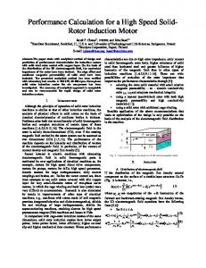
5. EXPERIMENTAL VALIDATION To validate the use of the proposed procedure for induction motor speed estimation, the simulation results have to be compared to those given by experimental tests. The experimental unit, is located at the "Research Unity of Industrial Process Control" (UCPI). The experimental set-up, depicted in figure 5, is composed of a 1 kW squirrel cage motor, a drake powder, inverters, a real time controller board of dSPACE DS1104 and interfaces which allow to measure the position, the angular speed, the currents, the voltages and the torque between the tested machine and the drake powder. The applied softwares are MATLAB-Simulink and Control Desk. Functions of a particular library give direct access from MATLAB script to the variables of the application program running on the dSPACE board. So, it is sufficient to develop the estimation algorithm with Simulink. The experimental stator currents, voltages and rotor speed, observed with Control Desk, are detected at every sampling instant. The specifications and parameters of the machine are the same as those used in computer simulation.

Figure 5: View of the experimental setup 5. 1. Experimental results with sensor To investigate the speed robustness, a step disturbance torque of 5Nm is applied at t=70s. Fig. 6 shows the reference and real rotor speed response due to step change command from 400 to -400 rpm. As evidenced by the testing results, the induction motor drive functions very well. It can be seen that the real speed converge to the real values very quickly.

140


Real motor speed Reference motor speed

Figure 6: Speed response due to step change command from 400 to -400 rpm at load

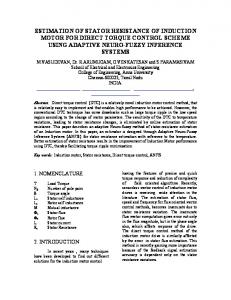
5. 2 Sensorless experimental results The actual machine model is used to calculate the current, flux, and speed of the motor. The adaptative algorithm as described above is used to estimate the stator flux and speed. Sensorless results are shown in Fig 7-8. The waveform of speed command , estimated and real speed obtained are shown in fig. 7 at no load. Fig. 8 shows the reference, estimated and real rotor speed response due to step change command from 1000 to -1000 rpm. As evidenced by the testing results, the induction motor drive functions very well by the proposed algorithm but a small fluctuations can be observed in speed estimation. There is still an error between the real stator flux and the estimation one obtained by the proposed method. In fact, the adaptative algorithm are dependent on the exact value of the machine parameters that are changeable with respect to the operating conditions. When the motor parameters are changed and, thus, are different from the preset values, the real speed will deviate from the reference values. The most influence parameter is the rotor résistance. In fact, it can increase by up to 50% relative to its value which is varying with temperature. This variation causes the misalignment of the actual and the estimated rotor flux. In fact, when the actual rotor resistance is larger or smaller than the estimated resistance, there will be more flux producing current and less torque producing current than the matched parameter case or less flux producing current and more torque-producing current than the matched parameter case respectively. To avoid this problem, a mutual estimation of rotor resistance and speed are necessary.

Reference motor speed Real motor speed Estimated motor speed

Figure 7: Transient response to speed command at no load

141


Reference motor speed Real motor speed Estimated motor speed

Figure 8: Real and estimated speed responses to speed step command 1000 to -1000rpm

6. CONCLUSION The MRAS technique was used to provide a real-time adaptive estimation of the motor speed. The practical modifications were carried out to implement the speed estimation and the validity with effectiveness of the proposed adaptation algorithm are verified by simulation and by experimental results. It has been shown both experimentally and theoretically that MRAS has satisfactory state observation capability for sensorless induction motor drive applications. Under operating conditions away from zero speed, the performance of the drive is very satisfactory. Some difficulties near zero speed require further research. REFERENCES [1]

Blasco-Giménez R., G. Asher, M. Summer, and K. Bradley, “Dynamic performance limitations for MRAS based sensorless induction motor drives. Part 1: Stability analysis for the closed loop drive,” Proc.IEE—Elect. Power Applicat., vol. 143, pp. 113–122, Mar. 1996.

[2]

Kim Y. R., S-K. Sul, and M. H. Park, “Speed sensorless vector control of an induction motor using an extended Kalman filter,” in Conf. Rec. IEEE-IAS Annu. Meeting, pp. 594–599, 1992.

[3]

Koubaa Y. et Mohamed Boussak, “Rotor resistance tuning for indirect stator flux oriented induction motor drive based on MRAS scheme,” Revue European Transactions on Electrical Power (ETEP)- Vol. 15, n°6, pp.557-570, 2005.

[4]

Koubaa Y., “Asynchronous machine parameters estimation using recursive method,” Journal Simulation Modelling Practice and theory (SIMPRA), Vol. 14 n°7, Elsevier Science, pp 10101021, 2006.

[5]

Kubota H., K. Matsuse and T. Nakano, “Dsp-based speed adaptive flux observer of induction motor,” IEEE Trans. Ind. Applicat., vol. 29, pp. 344–348, 1993.

[6]

Kubota H.and K. Matsuse, “Speed sensorless field-oriented control of induction motor with rotor resistance adaptation,” IEEE Trans. Ind. Applicat., vol. 30, pp. 1219–1224, 1994.

[7]

Lee C.M. and C. L. Chen, “Observer-based speed estimation method for sensorless vector control of induction motors,” Proc. IEE—Contr. Theory Applicat., vol. 145, pp. 359–363, May 1998.

[8]

Lee J.S., T. Takeshita and N. Matsui, ‘‘Stator-flux oriented sensorless induction motor drive for optimum low-speed performance,’’ IEEE Trans. Ind. Applicat. vol. 33, no. 5, pp. 1170–1176, 1997.

[9]

Lovati V., M. Marchesoni, M. Oberti and P. Segarich, ‘‘ A microcontroller-based sensorless stator-flux-oriented asynchronous motor drive for traction applications,’’ IEEE Trans. on Power Electron., vol. 13, no. 4, pp. 777– 785, 1988.

142

J. Electrical Systems 3-3 (2007): 131-143 [10] Jingchuan L., L. Xu, and Z. Zhang, ‘‘An adaptive sliding-mode observer for induction motor sensorless speed control,’’ IEEE Trans. Ind. Applicat. vol. 33, no. 5, pp. 1170–1176, 2005. [11] Peng Z.and T.Fukao, “Robust speed identification for speed sensorless vector control of induction motors,” IEEE Trans. Ind. Applicat., vol. 41, no. 4, pp. 1039–1047, 1994. [12] Schauder C., ‘‘ Adaptive speed identification for vector control of induction motors without rotational tranducers,’’ IEEE Trans. Ind. Appicat.., vol. 28, pp. 1054–1061, 1992. [13] Vas P., Sensorless Vector and Direct Torque Control. Oxford, U.K.: Oxford Univ. Press, 1998.

NOMENCLATURE

vds , vqs

d- and q-axis stator voltages.

ids , iqs

d- and q-axis stator currents.

idr , iqr

d- and q-axis rotor currents.

φds , φqs φdr , φqr

d- and q-axis stator flux linkages. d- and q-axis rotor flux linkages.

Rs , Rr stator and rotor resistances. Ls , Lr , M stator, rotor and mutual inductances.

ωr , ωsl , ωs p=

d dt

Te , Tl

rotor, slip and synchronous angular speed. Laplace, differential operator. electromagnetic and load torque.

J , f, σ Np τ r ,τ s

total inertia, friction total leakage coefficients. number of pole pairs. rotor and stator time constant.

^, *

denote the estimated and the reference values.

APPENDIX List of motor specification and parameters 220V, 1KW, 4 poles, 1430 rpm

Rs = 10Ω , Rr = 1.69Ω , Ls = 0.055H , Lr = 0.055 H , M = 0.049 H , f = 0.002 Nm

s / rad , J = 0.0035 Nm s 2 / rad

143