Salient Local Visual Features for Shape-Based 3D Model Retrieval - KKI

R. Ohbuchi, K. Osada, T. Furuya, T. Banno, Salient Local Visual Features for Shape-Based 3D Model Retrieval, accepted, Proc. IEEE International Conference on Shape Modeling and Applications (SMI’08), Stony Brook University, June 4 - 6, 2008.

Salient Local Visual Features for Shape-Based 3D Model Retrieval Ryutarou Ohbuchi

Kunio Osada

Takahiko Furuya

Tomohisa Banno

University of Yamanashi

University of Yamanashi

University of Yamanashi

University of Yamanashi

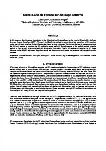
representation, e.g., watertight mesh. The invariance to noise and error in geometry and/or topology is important if similarity, not exact, matching is desired. This invariance to noise and error is also related to the invariance or tolerance to shape representation. The invariance to articulation, or pose change, of 3D models is addressed much less frequently than the other invariance mentioned above. Figure 1 shows examples of articulated 3D models. Using a typical shape comparison method, two models in the “human” class (or “snake” class) will not be very similar.

ABSTRACT In this paper, we describe a shape-based 3D model retrieval method based on multi-scale local visual features. The features are extracted from 2D range images of the model viewed from uniformly sampled locations on a view sphere. The method is appearance-based, and accepts all the models that can be rendered as a range image. For each range image, a set of 2D multi-scale local visual features is computed by using the Scale Invariant Feature Transform [22] algorithm. To reduce cost of distance computation and feature storage, a set of local features describing a 3D model is integrated into a histogram using the Bag-OfFeatures approach. Our experiments using two standard benchmarks, one for articulated shapes and the other for rigid shapes, showed that the methods achieved the performance comparable or superior to some of the most powerful 3D shape retrieval methods.

“human” class

“snake” class

KEYWORDS: Content-based retrieval, multi-scale feature, bag-offeatures, Scale Invariant Feature Transform.

Figure 1. Examples of articulated shapes found in the McGill University 3D shape benchmark database.

INDEX TERMS: H.3.3 [Information Search and Retrieval]: Information filtering. I.3.5 [Computational Geometry and Object Modeling]: Surface based 3D shape models. I.4.8 [Scene Analysis]: Object recognition.

In this paper, we propose a method for shape-based 3D model retrieval that performs well for both articulated and rigid models. The method also has a high degree of invariance to shape representation; the method accepts a diverse set of 3D shape representation so far as range image can be rendered. The method describes a 3D model by using a set of local, multi-scale, salient, visual features. The method first renders asset of range images of the model from multiple view directions about the model, as in the Light Field Descriptor (LFD) [5] or the Multiple-Orientation Depth Fourier Descriptor (MODFD) [25]. To extract local features from each range image, the proposed method uses the Scale Invariant Feature Transform (SIFT) algorithm proposed by Lowe [Lowe04]. As each depth image yields a few dozen features, and there are a few dozen range images per model, a 3D model is associated with thousands of local features. Computing dissimilarity between two sets of local features having thousands of local features each can be quite expensive. Assuming n features per model, comparing all the pairs of features of two models would cost O(n 2 ) . For a database of nontrivial size, such method would take too long to search. The cost of storing all the local features for large number of models per database is also very high. Our proposed method avoids the costly pair-wise distance computation by integrating all the local features of a model into a single feature vector by using the Bag-Of-Features (BoF) approach. The bag-of-features approach is inspired originally by the bag-of-words approach in text retrieval, which characterizes a text document by a histogram of words’ occurrences in the document. In our proposed method, vectorquantized local features, or visual words, from multiple range images are accumulated into single histogram to become a feature vector for the 3D model. The codebook for the vector quantization is learned via k-means clustering of local features extracted from the 3D models in the database. The bag-of-features approach is simple to implement, efficient to run, and as the experiments show, quite effective in retrieving 3D models.

1

INTRODUCTION

Three-dimensional (3D) models have become ubiquitous, for games running on mobile-phones and on game consoles, for such Web-based applications as the Google Earth, for medical diagnostics, and for mechanical or architectural design. The need to organize these 3D models, for example for effective reuse, has prompted research into shape-based retrieval of 3D models [35, 15]. A 3D shape comparison method must satisfy several requirements for invariance. A typical set of requirements includes (1) invariance to similarity transformations, (2) invariance to shape representations, (3) invariance to geometrical and topological noise, and (4) invariance to articulation or global deformation. Most of the 3D model retrieval methods try to satisfy the invariance to a certain class of geometrical transformation. The invariance to geometrical transformation can be gained by using a shape feature inherently invariant to the class of transformation, by using pose normalization, of by a combination of both. Some shape comparison methods are very tolerant of shape representations, accepting polygonal meshes, polygon soup, or even point sets. Others, however, assume certain shape †

4-3-11 Takeda, Kofu-shi, Yamanashi-ken, 400-8511, Japan. ohbuchiAT yamanashi.ac.jp, osada.researchAT gmail.com, t03kf030AT yamanashi.ac.jp, t01k073fAT yamanashi.ac.jp

1

R. Ohbuchi, K. Osada, T. Furuya, T. Banno, Salient Local Visual Features for Shape-Based 3D Model Retrieval, accepted, Proc. IEEE International Conference on Shape Modeling and Applications (SMI’08), Stony Brook University, June 4 - 6, 2008.

We have experimentally evaluated the proposed Bag-of-features SIFT (BF-SIFT) method. To evaluate retrieval performance for articulated models, we used the McGill 3D Shape Benchmark (MSB) [43]. To evaluate retrieval performance for rigid models, we used the Princeton Shape Benchmark (PSB) [30]. We compared the BF-SIFT with six other methods, which are, the Individual Match SIFT (IM-SIFT) algorithm, the LFD [5], the Spherical Harmonics Descriptor (SHD) [19], and our implementations of the D2 Shape Distribution [23], the Absolute Angle Distance histogram (AAD) [25], and the Surflet-Pair Relation Histograms (SPRH) [42]. Our experiments showed that the proposed BF-SIFT performed the best among those compared in retrieving articulated 3D models of the MSB. The BF-SIFT produced R-precision=75% for the MSB, compared to the LFD having R-Precision=57%. In retrieving rigid models, the BF-SIFT with R-Precision=45% performed comparably to the LFD (R-Precision=46%) or the SHD (R-Precision=40.5%). If we may summarize the contribution of this paper, they are: z z z

methods, however, are complex and difficult to compute under the presence of geometrical or topological error and noise. Another group of methods, e.g., the methods by Elad [7], Jain [16, 17], and Ran Gal [10, 11] uses curvature and other local geometrical and/or topological properties of manifold surfaces as the feature for pose invariant shape comparison. The method by Jain et al [Jain06, Jain07] employs a joint geometrical-topological analysis based on mesh spectral analysis for surface mesh models. These two classes of methods, however, are not applicable directly to many of the models used in computer graphics, e.g., polygon soup, meshes having multiple connected components, or point set models. For example, the method by Ran Gal et al [Gal07] in their paper evaluated their methods using only a subset of the PSB, since the method accepts only closed mesh that has single connected component and has no internal structure. Another class of approach employs segmentation to partition a model into “meaningful” sub-parts [34]. The method then extracts a feature form each sub-part for a part-based, pose-invariant retrieval. Due to the decomposition, however, the method could miss features associated with the relation of parts, for example, concavities in the shape. Yet another class of approaches uses a set of local features to achieve pose invariance for 3D model comparison [18, 2, 14, 34, 21, 31]. This class of method typically samples the surface of the model by using either 2D [18, 21, 2, 14] or 3D [31] local features. The 2D local feature based retrieval algorithms [2, 21] employ Spin Images algorithm by Johnson et al [18]. They sample the geometry by positioning cameras, e.g. cameras that capture images of vertices at numerous positions on the surfaces of the model [Johnson]. These images taken by the cameras are compared for shape matching. While powerful in their own rights, these methods have limitations. Using strictly a local feature, these methods miss global geometrical features. Consequently, their retrieval performances are low when applied to rigid models. The “distinctive regions” method by Shilane et al [31] used a multi-scale 3D feature centered at numerous locations of the model’s surface to sample local 3D geometrical features. This method is capable of capturing global as well as local feature, resulting in a good retrieval performance when applied to rigid model retrieval. Costs of feature comparison and feature storage are important issues for the methods based on local features. Assuming n features per model, comparing all the pairs of features of two models would cost O(n 2 ) . For a database of nontrivial size, such method would take too long to search thorough it. Cost of storage is significant also. A SIFT feature is a 128-dimensional vector, occupying 512Bytes per feature. A model containing 1,000 features requires 512kBytes to store the feature per model. To reduce these costs, a method could limit the area in the model B that is compared against a feature in the model A. This would work if the models have similar enough shapes and articulation (e.g., two standing human models) for correspondence and pose normalization. We used this approach in the Individual Match SIFT (IM-SIFT) algorithm described in Section 3.2. However, this approach would likely to fail if the models are completely different, or a model in a different articulation. In another approach by Shilne et al [31, for each sub-region of the 3D model to be compared, a small number of distinctive features are selected. The sub-region is found by essentially segmenting the model based on the similarity of local features within the subregion [31]. This distinctive regions approach is effective when evaluated for rigid model retrieval. Another, so-called bag-offeatures (BoF) approach is employed by Liu et al [21] for partial match retrieval of 3D models. The BoF approach integrates many

A new local, multi-scale, visual feature for 3D model retrieval that combines the SIFT [22] 2D image feature with the multi-view range-image renderings of 3D models. Successful application of the bag-of-features approach to 3D model retrieval that reduced the cost of feature storage and feature distance computation. Experimental evaluation of the proposed 3D model retrieval method compared to the other such methods by using a rigid model database and an articulated model database.

We will briefly review related work in the next section. Section 3 will describe our proposed method, and Section 4 will describe the experiments and their results. We will summarize the paper in Section 5. 2

RELATED WORK

Recently, there is an increasing body of work on 3D model retrieval. Please refer to survey papers [35, 15] and reports of recent 3D model retrieval contests [38, 39] for comprehensive lists. There are many requirements for a shape comparison method. Most of the time, geometrical transformation invariance of the method to at least similarity transformation is expected. Some methods, such as the D2 [23], the AAD [25], and the SPRH [42] are inherently invariant to similarity transformation. The SHD by Khazdan requires partial normalization of pose, in terms of position and scale, before the conversion from polygon-based model to voxel-based model is performed and a set of sphericalharmonic features is extracted. As the spherical harmonic feature rotation invariant, the SHD achieves invariant to similarity transformation. The LFD [5] and the MODFD [24] uses a different method to achieve rotation invariance. Both methods perform normalization of position and scale. The rotation invariance is achieved by the combination of multiple-view rendering of the object and a 2D image feature invariant to rotation in the image plane. While most of the published methods addressed the issue of geometrical transformation invariance, only a small minority of the methods addressed the issue of invariance to articulation or global deformation. For example, in most application scenarios, a human model would be considered the same if the figure is standing, running, or crouching. A group of methods that aim at articulation invariance uses topological approach to 3D shape comparison. Methods by Hilaga, et al [13] and by Tung et al [36] used extended Reeb graph. Methods by Biasotti [4] and Siddiqi et al [32] used medial-axis or skeleton-like representation and graph-based matching. These

2

R. Ohbuchi, K. Osada, T. Furuya, T. Banno, Salient Local Visual Features for Shape-Based 3D Model Retrieval, accepted, Proc. IEEE International Conference on Shape Modeling and Applications (SMI’08), Stony Brook University, June 4 - 6, 2008.

retrieving articulated models, It employs so-called “bag-offeatures” approach [33, 6, 9, 43] for the distance computation. The BF-SIFT perform pose normalization only for position and scale so that the model is rendered with an appropriate size in each of the multiple-view images. The BF-SIFT completely ignores the locations of local features for model similarity comparison. The IM-SIFT is aimed at retrieving rigid models. The IM-SIFT, on the other hand, tries to take advantage of positions of the local features in the pose-normalized model coordinate frame. Thus, the IM-SIFT performs full pose normalization, including scale, position, and rotation. By leveraging the positions of the features, it tries to avoid irrelevant comparison of local features. Avoidance of irrelevant comparison also reduces the cost of feature comparison, but not the cost of feature storage.

local features into a single feature vector [21], ignoring position of each feature. As the method used a single-resolution local feature, their method fails to capture global geometric shape of the models. The BoF approach is one of the most popular and powerful methods to compute distance among sets, or bags of features in the field of object recognition for 2D images [33, 6, 9, 43]. The BoF approach is inspired by the bag-of-words approach in text retrieval. Typically, the approach encodes a given local feature into one of several hundreds to thousands of visual word, by using a visual codebook. The visual codebook is often generated by performing k-means clustering on the set of local features by setting k to the size of vocabulary. Then, for each image, a histogram of visual words having the size of dictionary is created through vector quantization of local features. The histogram then becomes the feature vector for the image. Note that the locations of the local features in the image are not considered. A bicycle is a bicycle regardless of its position, orientation, or scale in the image. Our proposed method achieves transformation invariance by first performing partial pose normalization up to translation and scaling, followed by multiple-orientation rendering of the object coupled with 2D image features that are invariant to in-plane rotation. 3

3.1 BAG-OF-FEATURES SIFT ALGORITHM The BF-SIFT algorithm compares 3D models by following the steps below.

1.

METHOD

2.

In this section, we first describe the proposed 3D model comparison methods, Bag-of-Feature SIFT (BF-SIFT) algorithm. We also describe a similar algorithm based on multi-view local feature called Individual Match SIFT (IM-SIFT) algorithm. These two algorithms use the same multi-scale, multi-orientation, local, visual feature called Scale Invariant Feature Transform (SIFT) [22]. A combination of the SIFT feature, which is invariant to inplane rotation, with the multiple-orientation range-image rendering of 3D models to be compared achieves rotation invariance. Full pose invariance to similarity transformation is realized by normalizing scale and position of the models prior to the multiple-orientation range-image rendering. Our method produces tens to thousands of local features per 3D model. The number of features per 3D model depends on the 3D model to be compared, the number of images rendered of the model, and the parameters used to extract the SIFT feature, e.g., image size and the number of sub-bands per octave in the scale space. The BF-SIFT and the IM-SIFT differs in their ways to compute distance between two sets of visual features. The BF-SIFT aims at Render rangeimages from multiple views

Extract local visual features

… Number of views Ni

4.

5. 6.

Vector quantize features into visual words

Bag-offeatures

View 1

View i

3.

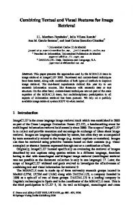
Pose normalization (position and scale): The BF-SIFT performs pose normalization only for position and scale so that the model is rendered with an appropriate size in each of the multiple-view images. Pose normalization is not performed for rotation. Multi-view rendering: Render range images of the model from Ni viewpoints placed uniformly on the view sphere surrounding the model. Local feature extraction: From the range images, extract local, multi-scale, multi-orientation, visual features by using the SIFT [Lowe04] algorithm. Vector quantization and histogram generation: Vector quantize a local feature into a visual word in a vocabulary of size N v by using a visual codebook. Prior to the retrieval, the visual codebook is learned, unsupervised, from thousands of features extracted from a set of models, e.g., the models in the database to be retrieved. Histogram generation: Quantized local features are accumulated into a histogram having N v bins, which becomes the feature vector of the corresponding 3D model. Distance computation: Dissimilarity among a pair of feature vectors (the histograms) is computed by using Kullback-Leibler divergence (KLD);

Generate a histogram

Feature vector

Bags-ofvisual words Histogram

…

View Ni

k clusters

⎛5⎞ ⎜ ⎟ ⎜7⎟ ⎜ 4⎟ ⎝ ⎠

Vocabulary size k

Figure 2. Generating a feature vector in the Bag-of-Feature SIFT algorithm. For each of the range images the 3D model viewed from multiple viewpoints, SIFT [Lowe04] algorithm extracts local visual features. Each local feature is vector quantized by using a visual codebook into a visual word. Frequency of visual word occurred in multiple range images are accumulated into a histogram per 3D model to be the feature vector.

3

R. Ohbuchi, K. Osada, T. Furuya, T. Banno, Salient Local Visual Features for Shape-Based 3D Model Retrieval, accepted, Proc. IEEE International Conference on Shape Modeling and Applications (SMI’08), Stony Brook University, June 4 - 6, 2008. n

D ( x, y ) =

∑ ( y − x ) ln x i

i =1

i

yi i

where x = ( xi ) , y = ( yi ) are the feature vectors and n is the dimension of the vectors. The KLD is sometimes referred to as information divergence, or relative entropy, and is not a distance metric, for it is not symmetric.

Figure 3. Cameras are placed at vertices of a polyhedron having either 6, 12, or 42 vertices, looking at the center of the polyhedron, for uniformly spaced (in terms of solid angle) view directions.

For pose normalization, the scale of the model is normalized by finding the smallest enclosing sphere, and the centroid of the model is placed at the global coordinate origin. The centroid is computed by using the quasi Monte-Carlo sampling of mass distribution on the surfaces of the model [25]. In rendering the multi-view range-images, the viewpoints are spaced evenly in the solid angle by placing them at vertices of regular or near-regular polyhedrons enclosing the model. In our experiments, we compared the numbers of views N i of 6, 20, and 42. Viewpoints are placed at the vertices of octahedron (6 vertices), icosahedron (20 vertices), and an 80-face (42 vertices) semi-regular polyhedron generated from the icosahedron by using Butterfly subdivision (Figure 3). The range-image rendering uses orthographic projection, and its front and rear clipping planes are set to tightly enclose the 3D model. The numbers of views N i are 6, 20, and 42 in our experiments. We used the range-image size of 2562 . After the range images are rendered, the SIFT algorithm is applied to each of the range images to detect interest points and then to compute features at these interest points. The SIFT algorithm first finds positions of features of what it thinks are salient. The saliency decision is based on a multi-scale, multiorientation, difference of Gaussian detector for gray-level changes, and each SIFT feature encodes these information. The salient points and features generated by the SIFT algorithm are more or less invariant to position, scale, orientation, and photometric (e.g., brightness) variances of the feature. The size of the SIFT descriptor is determined by a few parameters, such as the number of subdivision of the scale space and the size of bins that encode the orientation of the local feature. We set the parameters to their defaults, which produces a 128D vector as a feature. To compute the SIFT features, we used the C++ implementation named SIFT++ by Vedaldi [37]. The SIFT algorithm typically produces anywhere from ten to a few hundreds of local features per image, depending on the image. According to our experiments, the numbers of features extracted averaged over a database are; 37~38 per view for the MSB and 44~48 for the PSB. More features in the PSB models can be explained by the fact that the models in the PSB are more detailed and complex than those in the MSB. These numbers of features per range image means that a model is associated with thousands of local features. Using 42 views, a MSB model and a PSB model is associated with up to 1,500 and 2,000 SIFT features, respectively. Figure 5 shows the examples of SIFT interest points generated on four silhouette images that are sheared, rotated, and scaled. Interest points appear at similar locations in these four images in spite of the geometrical transformations. This robustness against geometric transformations appears to contribute to the 3D model retrieval performance. Note also that the interest points appear both inside and outside the body, detecting both concave and convex features. Segmentation approach such as [34] could miss many of these convex features.

Figure 4. Interest point detection and local visual feature extraction from range images rendered from multiple views (in this case six orthogonal views) by using Lowe’s SIFT algorithm [Lowe04].

Figure 5. Interest points of the SIFT algorithm are robust, to a certain degree, against various geometric transformations. Note also that the interest points appear inside and outside the body.

Each SIFT feature extracted from 3D models is vectorquantized into a visual word by using a visual codebook. To quantize, for each feature, we simply searched linearly through the codebook to find a visual word closest to the feature. The visual codebook is learned, unsupervised, prior to the retrieval by using k-means clustering of the features collected from every view of every model stored in the database. After the clustering, each cluster is represented by a representative code vector at the barycenter of the cluster. The k-means clustering requires quite significant spatial and computational cost when millions of

4

R. Ohbuchi, K. Osada, T. Furuya, T. Banno, Salient Local Visual Features for Shape-Based 3D Model Retrieval, accepted, Proc. IEEE International Conference on Shape Modeling and Applications (SMI’08), Stony Brook University, June 4 - 6, 2008.

features are to be processed. Thus the algorithm sub-samples the feature set down to 50,000 or 40,000 features. Once the vector quantization is done, frequencies of visual words generated from a model are accumulated into a histogram having N v bins. The histogram becomes the N v -dimensional feature vector for the 3D model, in which N v = 1,000 ~ 1,500 . A distance among a pair of feature vectors is computed by using the Kullback-Leibler divergence. The codebook learning via k-means clustering and vector quantization via linear search are expensive to compute. The kmeans clustering of 5 × 105 features with vocabulary size k=1,000 took about 2,500s, or 40 minutes. The vector quantization of the 5 × 105 features, or the feature for about 250 models, took about 7 minutes. Note, however, that these lengthy computations need only take place during the pre-processing stage, prior to the query sessions. For a query, the cost of computation is (1) extracting and vector quantizing about 2k features for the model, and, (2) computing a KLD distance par model pair using feature vectors having dimension of 1,000~1,500.

Monte-Carlo sampling the surfaces of the model with points having unit mass, the method we used for the AAD feature [25]. After the points are generated, a 3x3 covariance matrix of point distribution is computed. The eigenvectors of the covariance matrix becomes the principal axes of the model. The mass-PCA determines the orientation, but not the direction of the models. The position of barycenter relative to the center of the rectangular bounding box of the model determines the direction of the model in the normalized coordinate system. Another pose normalization method is called normal-PCA. It again performs PCA but this time on the surface normal orientation [29]. Oftentimes, the mass-PCA performs better than the normalPCA. However, there are occasions in which normal-PCA does better. Our method thus computes two distances using the two pose normalization methods, and merge the two at the last stage by taking the minimum of the two. Feature qi

3.2 INDIVIDUAL MATCH SIFT ALGORITHM The IM-SIFT assumes rigid models, and compare features extracted from “corresponding” areas in the pose-normalized global coordinate frame (Figure 6). To do this, the method performs full pose-normalization against similarity transformation. To improve performance, the IM-SIFT compute two independent distances using two pose normalization methods, and integrate the distance at the last stage by taking the minimum of the two distances. The IM-SIFT algorithm proceeds as follows;

1.

2. 3. 4.

5.

6.

Compare q with m nearest neighbour features in d.

Detail A close-up view. Model q

Model d

Figure 6. A feature in the model to the left is restricted to its proximity in the model to the right in the pose-normalized coordinate space. The correspondence assumes successful pose normalization, however.

Pose normalization (position, scale, and rotation): Pose normalization is performed for full similarity transformation, that is, for translation, (uniform) scaling, and rotation prior to rendering depth images. To normalize for rotation, either the mass-PCA or the normal-PCA is employed. These two rotation normalization methods are described later. If pose normalization is successful, “head to head” or “tire to tire” comparison of local features can be achieved for rigid models. Multi-view rendering: Same as in the BF-SIFT. Local feature extraction: Same as in the BF-SIFT. Feature dimension reduction: Prior to the feature-tofeature distance computation, the method performs feature dimension reduction on each SIFT feature using PCA [Ke04]. Distance computation: In the IM-SIFT algorithm, the perimage distance per pose normalization method is computed by individually matching local features in the image pair. The method computes, for each range image, the sum of individual L1 distance between a local feature pair. During the process, the method weighs the inter-image distance so that the image pair having significantly different number of feature points will have a larger distance. An overall distance between a pair of 3D models (per pose normalization method) is the sum of per-image distances. Distance integration: Two inter-3D-model distance values, one computed using the mass-PCA and the other computed using the normal-PCA, is integrated by taking the minimum of the two.

Figure 7. Examples of rotational pose normalization using the mass-PCA (avobe) and normal-PCA (below) methods. The massPCA is more successful in general but normal-PCA occasionally is better.

During the preliminary experiments, we compared the performances of several linear dimension reduction algorithms, the PCA, Indipendent Compondent Analysis (ICA) using the FastICA algorithm [8] and the Locality Preserving Projections (LPP) [12]. In the set of parameters we experimented, the PCA performed the best. We use the subspace dimension of the PCA at which the contribution from the subspace is 99%. In pairing local features for individual-match distance computations, we pair those features that lie close to each other in the pose normalized global coordinate frame. For each feature in a model, the algorithm picks k-nearest features for distance computation. This reduces the number of local-feature-to-local-

One of the pose normalization methods, called mass-PCA, is based on inertial moment of a mass uniformly distributed on the surfaces of the model [41]. We approximate the mass by quasi-

5

R. Ohbuchi, K. Osada, T. Furuya, T. Banno, Salient Local Visual Features for Shape-Based 3D Model Retrieval, accepted, Proc. IEEE International Conference on Shape Modeling and Applications (SMI’08), Stony Brook University, June 4 - 6, 2008.

feature distance computation from O(n 2 ) down to O( n ⋅ k ) , where n  k . In reality, pose normalizations fail, and a pair of 3D models may have no natural correspondence. In such cases the retrieval performance of the method won’t be high. When computing a distance among a pair of local features, the method increases the distance if the feature pair is extracted the image pair having a large discrepancy in the number of interest points. To do this, we multiply the inter-image distance by the following weight w;

precision, which is commonly used in the information retrieval literature [3]. In the first set of experiments, we evaluated the influence the number of views and the number of vocabulary size have on the retrieval performance. In the second set of experiments, we used the best performing of the BF-SIFT and IM-SIFT methods and compared their performance with those of several well-known (global) shape descriptors. 4.1

NUMBER OF VIEWS, VOCABULARY SIZE AND RETRIEVAL PERFORMANCE In the first set of experiments, we evaluated the influence the number of views Ni and the number of vocabulary size N v have on the retrieval performance. Figure 9a and Figure 9b show the results of experiments for the MSB and PSB, respectively. Retrieval performance is measured using R-precision. As mentioned above, for BF-SIFT, all but one of the codebooks are generated by clustering 50,000 features. We tried a larger training set size of 420,000 for the 42-view BF-SIFT (BF-SIFT-42*) retrieving MSB to see the effect of the training set size on the performance curve. Every one of the plots of the vocabulary size v.s. the performance has a peak; a retrieval performance suffers if the vocabulary size N v is either too small or too big. The peaks shift from left to right (toward larger vocabulary size) as the number of views increase from 6 to 42 and the total number of local features increases. We thus suspect that these peaks appeared probably because the number of feature points generated by the SIFT algorithm are not enough for each view. If we could somehow increase the number of local features per view, further increase in vocabulary size might have produced better overall retrieval performance. We observe that, for the MSB, the 20-view case clearly outperforms the 6-view case. But the 20-view and 42-view cases are very close in their maximum performance attained. The difference between the 20-view and the 42-view cases is the sharpness of the peaks; the 42-view case has a much broader peak than the 20-view case. In case of the PSB, the 42-view case clearly outperforms both the 6-view and the 20-view cases. This may be due to the greater diversity of shapes in the PSB compared to the MSB, which made a larger vocabulary preferable for the PSB. For the PSB also, a peak is much broader for a larger vocabulary size. The broader peak for a larger number of views (and thus a larger number of local features) may be explained as follows; with increasing number of views, a local visual feature tend to be described by multiple visual words so that the robustness increased. In Figure 9a for the MSB, we also list the performance curve for the visual codebook generated by clustering 420,000 features, instead of 50,000 features. Increasing the training set size Nt appears to slightly improve retrieval performance in this case. We need to investigate this aspect further. Note that the training set size can’t simply be increased; the larger the training set size, the more time the k-means requires to cluster the samples.

⎛ ( p − q )2 ⎞ ⎟ w = exp ⎜ ⎜ 2 max p , q 2 ⎟ ( ) ⎝ ⎠

where p and q are the local feature set for the two images taken from the same view, and p and q are the number of features in the pair of images.

Figure 8. An image pair having nor natural correspondence. The pair also has a large difference in the number of features.

4

EXPERIMENTS AND RESULTS

We experimentally evaluated the retrieval performance of our approach by using two benchmark databases: the McGill university benchmark database (MSB) [44] for articulated shapes and Princeton Shape Benchmark (PSB) [30] for a set of diverse, rigid shapes. The MSB consists of 255 models in 10 classes. The MSB include such articulated shapes as “human”, “octopus”, “snake”, “pliers”, and “spiders”. The PSB contains two equalsized subsets, the training set and test set, each consisting of 907 models and about 90 classes. For our evaluation, we used the PSB test set partitioned into 92 classes. The PSB contains a more diverse set of 3D shapes than the MSB. We used the same database for learning a visual codebook and for performance evaluations. That is, the codebook generated by using the MSB (PSB) is used to query the MSB (PSB). To generate visual codebook by using k-mean clustering, we used the training set size Nt = 50,000 SIFT features extracted from multiview images of models. There is an exception to this; we used Nt = 420,000 SIFT features generated using 42 views for the MSB models to see if the impact of training set size on the retrieval performance (See Section 4.1 for the details.) For both BF-SIFT and IM-SIFT, we used the images size of 256 × 256 pixels. As performance measures, we used R-precision and and recallprecision plot [Baeza-Yates99]. R-precision is a ratio, in percentile, of the models retrieved from the desired class Ck (i.e., the same class as the query) in the top R retrievals, in which R is the size of the class Ck . R-precision is in fact the same as the First-Tier measure used by Shilane, et al [PSB2004]. We use the term R-

4.2

PERFORMANCE COMPARISON WITH OTHER SHAPE DESCRIPTORS Figure 10 summarizes the retrieval performance of seven 3D model shape comparison algorithms evaluated by using both MSB (articulated figure) and PSB (rigid figure) benchmark databases. In Figure 10, the numbers for BF-SIFT and IM-SIFT are those of 42 views. The MSB-50k and MSB-420k generated the visual

6

R. Ohbuchi, K. Osada, T. Furuya, T. Banno, Salient Local Visual Features for Shape-Based 3D Model Retrieval, accepted, Proc. IEEE International Conference on Shape Modeling and Applications (SMI’08), Stony Brook University, June 4 - 6, 2008.

of the D2, AAD, and the SPRH are available online as Windows XP (32bit) executables at our web site [26]. Figure 11a and Figure 11b shows, for the MSB and PSB, respectively the recall-precision plots for the five shape descriptors, the BF-SIFT, IM-SIFT, D2, SHD, and LFD descriptors For the articulated models in the MSB, the proposed BF-SIFT with its R-Precision=75% outperformed, with a large margin, all the others we have compared against. The second place was the IM-SIFT-42 with R-Precision=64%, followed by the LFD and SHD in the third place with R-Precision=57%. Figure 8 also shows that the codebook learned from a larger (420,000) training set performed marginally better than the one learned from smaller number (50,000) of samples. By visual comparison of the recall-precision plots the IM-SIFT appears to perform comparably to the method for articulated model retrieval by Jain et al [16, 17]. An advantage of the BFSIFT over the method by Jain, et al is its capability to accept diverse shape representations, including polygon soup, point set, and B-rep solids. On the contrary, Jain’s method is directly applicable only to a singly connected mesh. Figure 12 shows retrieval examples for querying the MSB by the “snake” and “hand” models. In these examples, the retrieval results due to the BF-SIFT are clearly better than the LFD. For the generic, rigid models in the PSB, The LFD performed the best (R-precision=45.9%), followed closely by the proposed BF-SIFT-42 (R-precision=45.5%). It can be said that the BFSIFT-42 performs fairly, but not exceedingly, well in retrieving generic, rigid 3D models. Note also that, for the PSB, the IMSIFT-42 performed roughly as well as the BF-SIFT-42. The localfeature-in-global-context approach of the IM-SIFT appears to work well for the rigid models, but not for the articulated models.

80 70

R-Precision [%]

60 50 40 30 20

6 views 20 views 42 views 42 views (Nt=420000)

10 0 0

500

1000 1500 2000 Vocabulary size Nt

2500

3000

Figure 9a. Vocabulary size and retrieval performance of BF-SIFT for the MSB with three numbers of views. The codebook for the case marked by “Nt=420000” used 420,000 training features. All the other codebooks are generated by 50,000 training features.

80 70

R-Precision [%]

60 50

28.3

D2

40 30

33.2

AAD

20 10

500

1000 1500 2000 Vocabulary size Nt

53.9 45.9

LFD

0 0

56.3

37.3

SPRH

6 views 20 views 42 views

48.7

2500

3000

40.5

SHD

Figure 9b. Vocabulary size and retrieval performance of BF-SIFT for the PSB using three numbers of views. Codebook is generated by using 50,000 features.

56.7

44.7

IM-SIFT -42

64.2

45.5

BF-SIFT -42

codebooks by clustering 50,000 and 4200,000 samples, respectively. The other four fetures are global shape features. We implemented the D2 [23], AAD [25], and the SPRH [42] ourselves while the SHD [19] and the LFD [5] are computed by using the executables found on the web sites of the original authors of the papers. Our implementation of the D2 differs from that of Osada’s in some details, e.g., the use of quasi-random sequence and the number of bins. The details of the AAD are described in [25]. As the SPRH is originally developed for point set models, we borrowed the surface sampling step of the AAD to convert surface-based models into point set models. Our implementations

56.9

0

20

40

74.3 75.5 60

80

R-Precision [%] MSB-420k

MSB-50k

PSB

Figure 10. Retrieval performances, in R-precision [%], of the seven algorithms measured using both MSB (articulated figure) and PSB (rigid figure) databases.

7

R. Ohbuchi, K. Osada, T. Furuya, T. Banno, Salient Local Visual Features for Shape-Based 3D Model Retrieval, accepted, Proc. IEEE International Conference on Shape Modeling and Applications (SMI’08), Stony Brook University, June 4 - 6, 2008.

e.g., polygon soup and meshes having multiple connected components, the advantages of the BF-SIFT would become significant. The distinctive regions method by Shilane, et al reports First Tier performance for the PSB Test Set of 45.5%, which comparable to the that of the BF-SIFT-42 with its RPrecision=45.5%. (As mentioned before, R-precision and First Tier are the same.) We don’t know the performance of Shilane’s method [31] in retrieving the MSB. A comparison of our method with that of the method by Ran Gal, et al [11] is not possible, as his method accepts (without significant preprocessing) only a model that is watertight, has one connected component, and has no internal structure. As the PSB contains significant number of models that does not satisfy these conditions, the paper by Ran Gal reports results using only a “nicer” subset of the PSB using an undisclosed ground truth classifications. The Figure 10 also shows discrepancies of performance among shape features for retrieving models in the MSB and the PSB. For example, while the AAD lags far behind the LFD or SHD in retrieving PSB, the AAD almost tied the LFD and SHD in retrieving the MSB. The rand of the SPRH and the AAD actually reversed; while the SPRH did better for the PSB, the AAD did better for the MSB.

1

Precision

0.8

0.6

0.4 BF-SIFT-42* IM-SIFT-20 LFD SHD D2

0.2

0 0

0.2

0.4

0.6

0.8

1

Recall Figure 11a. Recall-precision plot for retrieving articulated shapes in the MSB.

5

1

Precision

0.8

0.6

0.4

0.2

0 0

0.2

0.4

0.6

0.8

SUMMARY AND FUTURE WORK

This paper proposed a powerful, computationally efficient algorithm for 3D model retrieval that handles both articulated and rigid models quite well. The method, named Bag-of-Features SIFT (BF-SIFT), employs a powerful 2D local image feature called Scale Invariant Feature Transform (SIFT) by Lowe [22]. The SIFT is invariant to translation, scaling, and rotation of features in 2D. The SIFT algorithm is applied to a set of multiple view depth images rendered from the 3D model to be compared, producing thousands of local visual features per model. Thanks to the multi-scale nature of the SIFT, the method captures both local and global shape features. To compute distance, the method employs the Bag-of-Features (BoF) approach that fuses all the local features into a single feature vector. The BoF approach vector-quantizes local features into visual words, and accumulates the frequency of the words into a histogram. The quantizer, or the codebook, is learned a priori by using a large set of local features extracted from the kind of models to be retrieved, e.g., the models in the database. The integration of thousands of local features into the feature vector reduced the cost of feature storage and the cost of feature comparison. We have experimentally evaluated the method by using the McGill Shape Benchmark (MSB) [44] of articulated 3D models and the Princeton Shape Benchmark (PSB) [30] of the rigid generic 3D models. The MSB contains only watertight meshes, while the PSB contains polygon soup models and non-manifold features. In retrieving articulated models in the MSB, the BF-SIFT performed the best. The proposed method have the RPrecision=75%, a value significantly higher than all the others. The IM-SIFT in the 2nd place had R-Precision=64.2% and the Light Field Descriptor (LFD) [5] in the 3rd place had RPrecision=56.9%. While a direct comparison was not performed, the proposed method appears to have comparable retrieval performance to the method by Jain et al for articulated models [Jain07] that uses mesh spectral analysis. In retrieving rigid models in the Princeton Shape Benchmark [30], the BF-SIFT with R-Precision=45% performed comparably

BF-SIFT-42 IM-SIFT-42 LFD SHD D2

1

Recall Figure 11b. Recall-precision plot for retrieving rigid shapes in the PSB.

In retrieving rigid model of the PSB, some of the recent methods, such as the SPRH feature combined with the multiresolution feature extraction and Semi-Supervised Dimension Reduction (SSDR) [27] with R-precision=53%, would outperform the LFD, the SHD, and the BF-SIFT-42. While direct comparison has not been made, other recent methods such as the one by Napoléon, et al [39] or the one by Akgul et al [1] would also outperform the BF-SIFT in retrieving the PSB. Overall, the BF-SIFT performed quite well for both articulated models in the MSB and the rigid models in the PSB. Unlike most of the global features, the BF-SIFT clearly excelled in retrieving articulated models in the MSB and performed on a par with some of the best method for articulated models know to us. If the retrieval task includes both articulated and rigid models, and the models to be retrieved include diverse set of shape representations,

8

R. Ohbuchi, K. Osada, T. Furuya, T. Banno, Salient Local Visual Features for Shape-Based 3D Model Retrieval, accepted, Proc. IEEE International Conference on Shape Modeling and Applications (SMI’08), Stony Brook University, June 4 - 6, 2008.

to the LFD (R-Precision=46%) or the local-feature based method by Shilane, et al [31] (R-Precision=46%). In the future, we would like to explore the approach further for a better retrieval performance and more efficient computation. For example, we would like to find a faster and more efficient codebook generation algorithm that is able to handle larger training set. Extraction of features of feature comparison may be accelerated further, e.g., by using a Graphics Processing Unit. We would also like to explore methods to solve the issue of occlusion so a complex shape or a shape having internal structure may be compared.

[18] A. E. Johnson, M. Hebert, Using Spin-Images for efficient multiple model recognition in cluttered 3-D scenes, IEEE Trans. on Pattern Analysis and Machine Intelligence, 21(5), pp. 433-449, (1999). [19] M. Kazhdan, T. Funkhouser, S. Rusinkiewicz, Rotation Invariant Spherical Harmonics Representation of 3D Shape Descriptors, Proc. Symposium of Geometry Processing 2003, pp. 167-175 (2003). [20] Y. Ke, R. Sukthankar, PCA-SIFT: A more distinctive representation for local image descriptors, Proc. CVPR 2004. [21] Y. Liu, H. Zha, H. Qin, Shape Topics: A Compact Representation and New Algorithms for 3D Partial Shape Retrieval, Proc. CVPR 2006, Vol. II, pp. 2025-2032, (2006) [22] D.G. Lowe, Distinctive Image Features from Scale-Invariant Keypoints, Int’l Journal of Computer Vision, 60(2), Nov. 2004. [23] R. Osada, T. Funkhouser, Bernard Chazelle, and David Dobkin, Shape Distributions, ACM TOG, 21(4), pp. 807-832 (2002) [24] R. Ohbuchi, M. Nakazawa, T. Takei, Retrieving 3D Shapes Based On Their Appearance, Proc. ACM MIR 2003, pp. 39-46, (2003). [25] R. Ohbuchi, T. Minamitani, T. Takei, Shape-similarity search of 3D models by using enhanced shape functions, International Journal of Computer Applications in Technology (IJCAT), 23(3/4/5), pp. 70-85, 2005. [26] R. Ohbuchi’s web page, http://www.kki.aymanashi.ac.jp/~ohbuchi/research_index.html [27] R. Ohbuchi, A. Yamamoto, J. Kobayashi, Learning semantic categories for 3D Model Retrieval, Proc. ACM MIR 2007, pp. 31-40, (2007). [28] W. H. Press et al., Numerical Recipes in C-The Art of Scientific Programming, 2nd Ed., Cambridge University Press, Cambridge, UK, 1992. [29] J. Pu, K. Lou, K. Ramani, A 2D Sketch-Based User Interface for 3D CAD Model Retrieval, Computer Aided Design and Application, 2(6), pp.717-727, (2005). [30] P. Shilane, P. Min, M. Kazhdan, T. Funkhouser, The Princeton Shape Benchmark, Proc. SMI ‘04, pp. 167-178, (2004). http://shape.cs.princeton.edu/search.html [31] P. Shilane, T. Funkhouser, Distinctive Regions of 3D Surfaces, ACM Trans. Graphics, 26(2), (2007). [32] K. Siddiqi, J. Zhang, D. Macrini, A. Shokoufandeh, S. Bioux, and S. Dickinson, Retrieving Articulated 3-D Models Using Medial Surfaces, Machine Vision and Applications, Springer Online First as of September 2, 2007. [33] J. Sivic, A. Zisserman, Video Google: A text retrieval approach to object matching in Videos, Proc. ICCV 2003, Vol. 2, pp. 1470-1477, (2003) [34] A. Tal, E. Zuckerberger, Mesh retrieval by components, Proc. GRAPP 2006, pp. 142-149, (2006). [35] J. Tangelder, R. C. Veltkamp, A Survey of Content Based 3D Shape Retrieval Methods, Proc. SMI '04, pp. 145-156. [36] T. Tung, F. Schmitt, Augmented Reeb Graphs for Content-based Retrieval of 3D Mesh Models, Proc. SMI '04, pp.157-166, (2004). [37] A. Vedaldi, SIFT++ A lightweight C++ implementation of SIFT, http://vision.ucla.edu/~vedaldi/code/siftpp/siftpp.html [38] R. C. Veltkamp, et al., SHREC2006 3D Shape Retrieval Contest, Utrecht University Dept. Information and Computing Sciences Technical Report UU-CS-2006-030 (ISSN: 0924-3275) [39] R.C. Veltkamp, F.B. ter Harr, SHREC 2007 3D Shape Retrieval Contest, Dept of Info and Comp. Sci., Utrecht University, Technical Report UU-CS-2007-015. [40] D. Vranić, D. Saupe, J. Rchter, Tools for 3D-object retrieval: Karhunen-Loeve transform and spherical harmonics. Proc. IEEE 4th Workshop on Multimedia Signal Processing, pp.293-298, (2001) [41] D. V. Vranić, 3D Model Retrieval, Ph.D. Thesis, University of Leipzig, 2004. http://merkur01.inf.uni-konstanz.de/CCCC/

ACKNOWLEDGEMENTS

The authors would like to thank those who carefully reviewed the paper. The authors also would like to thank those who created benchmark databases and those who made available codes for their shape features. This research has been funded in part by the Ministry of Education, Culture, Sports, Sciences, and Technology of Japan (No. 17500066 and No. 18300068). REFERENCES [1] [2] [3] [4]

[5]

[6]

[7] [8] [9]

[10] [11]

[12]

[13]

[14]

[15]

[16] [17]

C. V. Akgül, B. Sankur, F. Shmitt, Y. Yemez, Multivariate DensityBased 3D Shape Descriptors, Proc. SMI’07, pp.3-12, (2007). J. Assfalg, A. Del Bimbo, P. Pala, Retrieval of 3D Objects by Visual Simialarity, Proc. ACM MIR’04, pp. 77-83. R. Baeza-Yates, B. Ribiero-Neto, Modern information retrieval, Addison-Wesley (1999). S. Biasotti, S. Marini, M. Spagnuolo, B. Falcidieno, Sub-part correspondence by structural descriptors of 3D shapes, CAD, 38, pp.1002-1019, (2006). D-Y. Chen, X.-P. Tian, Y-T. Shen, M. Ouh-young, On Visual Similarity Based 3D Model Retrieval, Computer Graphics Forum, 22(3), pp. 223-232, (2003). G. Csurka, C.R. Dance, L. Fan, J. Willamowski, C. Bray, Visual Categorization with Bags of Keypoints, Proc. ECCV ’04 workshop on Statistical Learning in Computer Vision, pp.59-74, (2004) A. Elad, R. Kimmel, On bending invariant signatures for surfaces, IEEE Trans. on PAMI, 25(10), pp.1285-1295, (2003). FastICA implementation, http://www.cis.hut.fi/projects/ica/fastica. R. Fergus, L. Fei-Fei, P. Perona, A. Zisserman, Learning object categories from Google’s image search, Proc. ICCV’05, Vol. II, pp.1816-1823, (2005) R. Gal, D. Cohen-Or, Salient Geometric Features for Partial Shape Matching and Similarity, ACM TOG, 25(1), pp. 130-150, (2006) R. Gal, A. Shamir, D. Cohen-Or, Pose-Oblivious Shape Signature, IEEE Trans. Vis. Comp. Graph., 13(2), pp. 261-271, March/April 2007. X. He, P. Niyogi: Locality Preserving Projections, Advances in Neural Information Processing Systems 16, Vancouver, Canada, 2003. H. Hilaga, Y. Shinagawa, T. Komura, T. Kunii, Topology matching for fully automatic similarity estimation of 3D shapes, Proc. SIGGRAPH 2001, pp.201-212, (2001). D. Huber, A. Kapuria, R. R. Donamukkala, M. Hubert, Parts-based 3-d object classification, Proc. IEEE CVPR 2004, II-82 - II-89 Vol.2, (2004) M. Iyer, S. Jayanti, K. Lou, Y. Kalyanaraman, K. Ramani, Three Dimensional Shape Searching: State-of-the-art Review and Future Trends, Computer Aided Design, 5(15), pp. 509-530, (2005). V. Jain, H. Zhang, Robust 3D Shape Correspondence in the Spectral Domain, Proc. SMI’06, pp.19-28, (2006). V. Jain, H. Zhang, A spectral approach to shape-based retrieval of articulated 3D models, Computer Aided Design, 39, pp.298-407, (2007)

9

R. Ohbuchi, K. Osada, T. Furuya, T. Banno, Salient Local Visual Features for Shape-Based 3D Model Retrieval, accepted, Proc. IEEE International Conference on Shape Modeling and Applications (SMI’08), Stony Brook University, June 4 - 6, 2008. [44] J. Zhang, R. Kaplow, R. Chen, K. Siddiqi, The McGill Shape Benchmark (2005). http://www.cim.mcgill.ca/shape/benchMark/

[42] E. Wahl, U. Hillenbrand, G. Hirzinger, Surflet-Pair-Relation Histograms: A Statistical 3D-Shape Representation for Rapid Classification, Proc. 3DIM 2003, pp. 474-481, (2003). [43] J. Winn, A. Criminisi, T. Minka, Object categorization by learned universal visual dictionary, Proc. ICCV05, Vol. II, pp.1800-1807, (2005).

Qurey

BF-SIFT with 42 views

9

9

9

9

9

9

9

9

9

9

9

9

9

9

9

×

9

×

9

9

9

×

×

×

LFD “snake”

(a) Querying the “snake” class. Query

BF-SIFT with 42 views

9

9

9

9

9

9

9

9

9

9

9

9

9

9

9

×

×

×

×

×

×

×

9

×

LFD “hand”

(b) Querying the “hand” class. Figure 12. Retrieval results using the McGill articulated shape benchmark database (MSB). Retrieval results are shown in 2 by 6 matrix in which models are ordered left-to-right, top-to-bottom, by their similarity to the query to the left. In these examples, the BF-SIFT-42 clearly outperforms the Light Field Descriptor [5].

10