Jul 20, 2013 - [Erns 95] U. Ernst, K. Pawelzik, and T. Geisel. “Synchronization Induced by Tempo- .... [Rudi 76] W. Rudin. Principled of Mathematical Analysis.
Johannes Klinglmayr Matr.-Nr. 0201874
Self-Organizing Network Synchronization: Convergence and Robustness in Pulse-Coupled Oscillator Systems DISSERTATION zur Erlangung des akademischen Grades Doktor der technischen Wissenschaften Alpen-Adria-Universit¨ at Klagenfurt Fakult¨ at f¨ ur Technische Wissenschaften Begutachter: Univ.-Prof. Dr.-Ing. Christian Bettstetter Institut f¨ ur Vernetzte und Eingebettete Systeme Alpen-Adria-Universit¨at Klagenfurt Prof. Dr. Marc Timme Max-Planck Institut f¨ ur Dynamik und Selbstorganisation Georg-August-Universit¨at G¨ottingen
July 2013
Declaration of honor I hereby confirm on my honor that I personally prepared the present academic work and carried out myself the activities directly involved with it. I also confirm that I have used no resources other than those declared. All formulations and concepts adopted literally or in their essential content from printed, unprinted or Internet sources have been cited according to the rules for academic work and identified by means of footnotes or other precise indications of source. The support provided during the work, including significant assistance from my supervisor has been indicated in full. The academic work has not been submitted to any other examination authority. The work is submitted in printed and electronic form. I confirm that the content of the digital version is completely identical to that of the printed version. I am aware that a false declaration will have legal consequences.
(Signature)
(Place, date)
iii
Abstract Agreeing on a common timing (synchronization) is beneficial for distributed entities in a large number of applications. For instance, it enables synchronized distributed measurements to track moving objects or the scheduling of communication in wireless communication systems. Yet, how to provide synchronization for distributed systems in a reliable way remains an open challenge: Communication between individual entities is often subject to different individual delays, the network might be sparse, and clocks might not be homogeneous. A promising approach to synchronize a network of distributed entities is by only using local interactions and to communicate as little as possible, for instance by exchanging pulse-like messages, which do not contain information. It is well known that self-organizing processes may induce global synchronization via local interactions, e.g. if all entities act individually by the same rules. How to design these local rules to guarantee global synchronization, however, remains not well understood. So far, a general statement that guarantees global synchronization from local pulseinteractions could not be achieved if facing the challenges mentioned above. In this thesis we derive local interaction rules and mathematically guarantee global synchronization using pulse-coupled oscillator networks. Specifically, we provide two coupling schemes that address different system settings and prove network-wide convergence to synchrony. These proofs hold for systems which face individual random signal delays, inhomogeneous clock rates, arbitrary topologies, and stochastic pulse emission. We also show the robustness of the synchronization process in case of faulty or random pulse detection, incorrect assumptions about the environment and inaccurate oscillators. We apply the self-organizing synchronization to wireless communication systems. We demonstrate that the local interaction rules derived, enable self-organizing synchronization in wireless communication systems. In our proof-of-concept applications, we address distributed devices which use communication protocols with time slots. These slots are then used for data communication. The devices exchange pulse-like radio or audio signals and are designed to synchronize their time slots. This insight on local interaction rules helps to better understand self-organizing processes in a more general setting, including engineering and social sciences.
v
Zusammenfassung Eine zeitliche Anordnung verteilter Elemente ist f¨ ur viele Anwendungen von Vorteil. So l¨asst sich zum Beispiel mit der Verwendung synchronisierter Uhren ein bewegtes Objekt durch verteilte Beobachtungen verfolgen oder eine Kommunikationsvorschrift in drahtlosen Netzwerken koordinieren. Trotz vieler Anwendungsm¨oglichkeiten steht die zuverl¨assige Synchronisation von verteilten Systemen noch vor Herausforderungen: Bei der Kommunikation zwischen einzelnen Elementen entstehen oft unterschiedliche Verz¨ogerungen, das Kommunikationsnetz besteht oft aus nur wenigen Verbindungen und die Uhren in den verteilten Elementen haben oft nicht die selbe Geschwindigkeit. Nur lokale Kommunikation zuzulassen und diese auf ein Minimum zu reduzieren ist ein vielversprechender Ansatz um verteilte Systeme zu synchronisieren. Das gelingt beispielsweise durch die Verwendung von puls¨ahnlichen Nachrichten, die keinerlei Information beinhalten. Selbstorganisation ist eine M¨oglichkeit, um mithilfe lokaler Interaktion globale Synchronisation zu erzeugen. Dabei k¨onnen individuelle Elemente unter Ber¨ ucksichtigung der gleichen Interaktionsregeln selbst¨andig handeln. Wie genau das Design f¨ ur solche lokalen Interaktionsregeln auszusehen hat, um globale Synchronisation zu garantieren, ist noch nicht g¨anzlich verstanden. Unter Einbeziehung obiger Herausforderungen konnte eine generelle Aussage zur garantierten globalen Synchronisation durch lokale puls¨ahnliche Interaktionen bis dato nicht getroffen werden. Diese Arbeit zeigt lokale Interaktionsregeln auf und garantiert, mittels mathematische Beweisf¨ uhrung, globale Synchronisation pulsgekoppelter Oszillatornetzwerke. Im Speziellen werden zwei Kopplungsmethoden vorgestellt, die f¨ ur unterschiedliche Rahmenbedingungen globale Synchronisation garantieren. Sie gelten f¨ ur Systeme mit unterschiedlicher individueller Verz¨ogerung, unterschiedlicher Geschwindigkeit der Oszillatoren, beliebigen Netzwerken und stochastischer Puls¨ ubertragung. Dar¨ uber hinaus wird gezeigt, dass die so erreichte Synchronisation robust hinsichtlich zuf¨alliger und falscher Pulsdetektion und resilient hinsichtlich f¨alschlicher Randbedingungsannahmen und ungenauer Oszillatoreigenschaften ist. Diese Arbeit demonstriert die Umsetzung der vorgestellten selbstorganisierenden Synchronisationsmethoden in Kommunikationsnetzwerken. F¨ ur Kommunikationsmethoden mit Sendeintervallen zeigen die Implementationen die Konzepttauglichkeit der garantierten Synchronisationsmethoden. Sie beinhalten Ausf¨ uhrungen auf Standardger¨aten und auf programmierbarer Hardware. Eine interaktive Demonstration veranschaulicht die Nutzung selbstorganisierender Synchronisation mittels Audiosignalen. Durch diese Arbeit konnten neue Einsichten, das Design und die Dynamik lokaler Interaktionen betreffend, erlangt werden, die helfen, Selbstorganisation auch in einem breiteren Anwendungsfeld zu verstehen.
vii
Acknowledgements I would like to thank my advisor Prof. Dr-Ing. Christian Bettstetter. You drew my attention onto the field of self-organization, which since fascinates me. Your guidance and trust allowed me to focus on the mathematics in wireless communications. I would also like to thank my second advisor Prof. Dr. Marc Timme who taught me how to connect the worlds – of physics, reality and wireless communications. Reality might easily come off hands, if there were no colleagues. A huge thanks to my colleagues in Klagenfurt, above all Evsen, Torsten and Kornelia, who always had an open ear for my situations. Your good advice which often ending with “You never know what it is good for” will stay with me. Also thanks to my colleagues in G¨ottingen, above all Christian and Christoph. Your motivation for research always kept me up-beat and our discussions about the big picture will help me find the right way through life. This way through life has been encircled with friends, for whom I am deeply thankful. Thanks to all of you who distracted me from work, who joined me enjoying sun, mountain tops, snow, and the colors of life. Life has a lot of colors and those who always were by my side are my family. Thank you for your unconditioned support and hugs. Above all, thanks to my wife. You are my whirling soul of sunshine.
ix
Contents 1 Introduction 1.1 Principles of Self-Organizing Synchronization . . . . . . . . . . . . . . 1.2 Examples for Synchronization in Pulse-Coupled Oscillators . . . . . . 1.3 Self-Organizing Synchronization for Wireless Communication Systems 1.4 Pulses for Synchronization in Wireless Communication Systems . . . 1.5 Guarantees as Contribution to PCO Synchronization . . . . . . . . . 1.6 Structure of the Thesis . . . . . . . . . . . . . . . . . . . . . . . . . .
. . . . . .
2 Background on Synchronization 2.1 Synchronization in Wireless Communication Systems . . . . . . . . . . 2.1.1 Synchronization . . . . . . . . . . . . . . . . . . . . . . . . . . . 2.1.2 Wireless Communication Systems . . . . . . . . . . . . . . . . . 2.1.3 Benefits of Synchronization . . . . . . . . . . . . . . . . . . . . 2.1.4 Types of Synchronization for Wireless Communication Systems 2.1.5 Applications for Slot Synchronization . . . . . . . . . . . . . . . 2.1.6 Self-Organizing Synchronization . . . . . . . . . . . . . . . . . . 2.2 Networks of Pulse-Coupled Oscillators . . . . . . . . . . . . . . . . . . 2.2.1 Definition of an Oscillator . . . . . . . . . . . . . . . . . . . . . 2.2.2 Pairwise Interaction of Oscillators . . . . . . . . . . . . . . . . . 2.2.3 Interaction of an Ensemble of Oscillators . . . . . . . . . . . . . 2.2.4 Circular Representation . . . . . . . . . . . . . . . . . . . . . . 2.2.5 Delayed Pulses . . . . . . . . . . . . . . . . . . . . . . . . . . . 2.2.6 Synchronization of Oscillators . . . . . . . . . . . . . . . . . . . 2.2.7 Observations on the Synchronization Process . . . . . . . . . . . 2.2.8 Other Applications of Pulse-Coupled Oscillators . . . . . . . . . 2.3 Synchronization of Pulse-Coupled Oscillators . . . . . . . . . . . . . . . 2.3.1 Generalizations on Delays . . . . . . . . . . . . . . . . . . . . . 2.3.2 Synchronization in Arbitrary Connected Networks . . . . . . . . 2.3.3 Self-Organizing Synchronization for Wireless Communications . 2.4 Design Principles for Self-Organizing Synchronization . . . . . . . . . . 2.4.1 Modeling Approach . . . . . . . . . . . . . . . . . . . . . . . . . 2.4.2 Designing Update Functions for Synchronization . . . . . . . . . 2.4.3 Synchronization Strategies . . . . . . . . . . . . . . . . . . . . .
. . . . . .
1 1 1 2 3 4 5
. . . . . . . . . . . . . . . . . . . . . . . .
7 7 7 8 8 9 11 12 13 13 14 15 18 18 19 20 20 22 23 25 25 28 28 29 29
xi
Contents 3 Synchronization with Inhibitory Coupling 3.1 Motivation . . . . . . . . . . . . . . . . . . . . . . . . . . . . 3.1.1 Beneficial Synchronizing Effects . . . . . . . . . . . . 3.1.2 Outline of the Proof . . . . . . . . . . . . . . . . . . 3.2 Specifying the System Settings . . . . . . . . . . . . . . . . . 3.2.1 Oscillator Properties . . . . . . . . . . . . . . . . . . 3.2.2 Oscillator Coupling . . . . . . . . . . . . . . . . . . . 3.2.3 Refractory Interval . . . . . . . . . . . . . . . . . . . 3.2.4 Alternative Circular Representation . . . . . . . . . . 3.2.5 Leading Oscillator . . . . . . . . . . . . . . . . . . . 3.2.6 Sample Synchronization Process . . . . . . . . . . . . 3.3 Prerequisites . . . . . . . . . . . . . . . . . . . . . . . . . . . 3.3.1 Definition of Precision . . . . . . . . . . . . . . . . . 3.3.2 Steady State . . . . . . . . . . . . . . . . . . . . . . . 3.3.3 Approach for the Convergence Proof . . . . . . . . . 3.3.4 Properties of the System . . . . . . . . . . . . . . . . 3.4 Synchronization Convergence for Two Oscillators . . . . . . 3.5 Synchronization Convergence for an Ensemble of Oscillators 3.6 Performance and Robustness . . . . . . . . . . . . . . . . . . 3.6.1 Normalized Precision for Fair Comparisons . . . . . . 3.6.2 Simulation Setup . . . . . . . . . . . . . . . . . . . . 3.6.3 Synchronization Performance . . . . . . . . . . . . . 3.6.4 Robustness . . . . . . . . . . . . . . . . . . . . . . . 3.7 Inhibitory Coupling in Meshed Networks . . . . . . . . . . . 3.8 Summary . . . . . . . . . . . . . . . . . . . . . . . . . . . .
. . . . . . . . . . . . . . . . . . . . . . . .
. . . . . . . . . . . . . . . . . . . . . . . .
. . . . . . . . . . . . . . . . . . . . . . . .
. . . . . . . . . . . . . . . . . . . . . . . .
. . . . . . . . . . . . . . . . . . . . . . . .
. . . . . . . . . . . . . . . . . . . . . . . .
. . . . . . . . . . . . . . . . . . . . . . . .
31 31 31 32 33 33 33 34 35 36 36 38 38 38 39 39 41 44 47 48 48 49 50 56 57
4 Synchronization with Inhibitory and Excitatory Coupling 4.1 Motivation . . . . . . . . . . . . . . . . . . . . . . . . . 4.2 System Settings . . . . . . . . . . . . . . . . . . . . . . 4.2.1 Network . . . . . . . . . . . . . . . . . . . . . . 4.2.2 Oscillators . . . . . . . . . . . . . . . . . . . . . 4.2.3 Prerequisites . . . . . . . . . . . . . . . . . . . . 4.3 Proof of Convergence . . . . . . . . . . . . . . . . . . . 4.3.1 Properties of the System . . . . . . . . . . . . . 4.3.2 Synchronization Condition . . . . . . . . . . . . 4.3.3 Inevitability . . . . . . . . . . . . . . . . . . . . 4.3.4 Bounds for Further Generalizations . . . . . . . 4.4 Performance and Robustness . . . . . . . . . . . . . . . 4.4.1 Simulation Setup . . . . . . . . . . . . . . . . . 4.4.2 Impact of Network Size and Node Degree . . . . 4.4.3 Impact of Synchronization Bound . . . . . . . . 4.4.4 Impact of Dynamically Changing Networks . . . 4.4.5 Impact of the Pulse Emission Probability . . . . 4.4.6 Robustness to Delay Spread Assumptions . . . .
. . . . . . . . . . . . . . . . .
. . . . . . . . . . . . . . . . .
. . . . . . . . . . . . . . . . .
. . . . . . . . . . . . . . . . .
. . . . . . . . . . . . . . . . .
. . . . . . . . . . . . . . . . .
. . . . . . . . . . . . . . . . .
59 59 63 63 63 64 66 66 68 72 73 74 75 75 76 76 77 77
xii
. . . . . . . . . . . . . . . . .
. . . . . . . . . . . . . . . . .
. . . . . . . . . . . . . . . . .
Contents
4.5
4.4.7 Comparison with Pagliari-Scaglione Approach . . . . . . . . . . . 4.4.8 Robustness to Noise . . . . . . . . . . . . . . . . . . . . . . . . . Summary . . . . . . . . . . . . . . . . . . . . . . . . . . . . . . . . . . .
5 Proof of Concept in Wireless Networks 5.1 Network Synchronization without Sync-Word Detector 5.1.1 Pulse-Like Signal Detection . . . . . . . . . . . 5.1.2 Phase Updates and Cycles . . . . . . . . . . . . 5.1.3 Pulse Emission . . . . . . . . . . . . . . . . . . 5.1.4 Test-Bed Setup . . . . . . . . . . . . . . . . . . 5.1.5 Demonstration . . . . . . . . . . . . . . . . . . 5.1.6 Summary . . . . . . . . . . . . . . . . . . . . . 5.2 Network Synchronization with Sync-Word Detector . . 5.2.1 Pulse-Like Signal Detection . . . . . . . . . . . 5.2.2 Phase Updates and Cycles . . . . . . . . . . . . 5.2.3 Test-Bed Setup . . . . . . . . . . . . . . . . . . 5.2.4 Demonstration . . . . . . . . . . . . . . . . . . 5.2.5 Summary . . . . . . . . . . . . . . . . . . . . . 5.3 Network Synchronization with Audio Signals . . . . . . 5.3.1 Pulse-Like Signal Detection . . . . . . . . . . . 5.3.2 Phase-Updates and Cycles . . . . . . . . . . . . 5.3.3 Pulse Emission . . . . . . . . . . . . . . . . . . 5.3.4 Test-Bed Setup . . . . . . . . . . . . . . . . . . 5.3.5 Demonstration . . . . . . . . . . . . . . . . . . 5.3.6 Summary . . . . . . . . . . . . . . . . . . . . . 5.4 Synchronization Bounds in Practice . . . . . . . . . . .
. . . . . . . . . . . . . . . . . . . . .
. . . . . . . . . . . . . . . . . . . . .
. . . . . . . . . . . . . . . . . . . . .
. . . . . . . . . . . . . . . . . . . . .
. . . . . . . . . . . . . . . . . . . . .
. . . . . . . . . . . . . . . . . . . . .
. . . . . . . . . . . . . . . . . . . . .
. . . . . . . . . . . . . . . . . . . . .
. . . . . . . . . . . . . . . . . . . . .
. . . . . . . . . . . . . . . . . . . . .
78 79 82 85 86 87 87 87 88 88 90 90 90 92 92 92 92 94 95 95 96 96 96 96 97
6 Conclusions
99
List of Symbols
105
List of Own Publications
109
Bibliography
113
Curriculum Vitae
121
xiii
List of Tables 2.1 2.2 2.3
Phase evolution of oscillators as in Example 1. . . . . . . . . . . . . . . . Phase evolution of oscillators as in Example 2. . . . . . . . . . . . . . . . Phase evolution and phase ordering of oscillators as in Example 3. . . . .
23 24 25
3.1 3.2 3.3 3.4
Phase evolution of oscillators i and j . . . . . . . . . . . Parameter values for the simulations in Section 3.6. . . Steady state mean precision and precision bounds. . . . . Phase evolution of oscillators 1, 2 and 3 from Example 6.
42 49 49 56
6.1
Selected convergence proofs on self-organizing synchronization on pulsecoupled oscillators. . . . . . . . . . . . . . . . . . . . . . . . . . . . . . . 102
. . . .
. . . .
. . . .
. . . .
. . . .
. . . .
. . . .
. . . .
. . . .
xv
List of Figures 2.1 2.2 2.3 2.4 2.5 2.6 2.7 2.8 2.9
Three examples of communication protocols. . . . . . . . . . . . . . . . . Two representations of the phase evolution. . . . . . . . . . . . . . . . . Examples of the two different phase jumps according to the coupling scheme. System dynamics emerging from different coupling schemes. . . . . . . . Example of a graph G. . . . . . . . . . . . . . . . . . . . . . . . . . . . . An example of the effect of individual random delays. . . . . . . . . . . . An example of the distance as defined in (2.16). . . . . . . . . . . . . . . The two possible modes of an oscillator within the MEMFIS algorithm. . The two possible modes within the PCO protocol. . . . . . . . . . . . . .
3.1
3.13
Update function and phase evolution with inhibitory coupling and selfadjustment. . . . . . . . . . . . . . . . . . . . . . . . . . . . . . . . . . . Circular phase representation, using p(φ) from (2.13), with inhibitory coupling as defined in (3.2) and (3.3). . . . . . . . . . . . . . . . . . . . . Alternative circular representation using p˜(φ) from (3.5). . . . . . . . . . The index permutation of the oscillators. . . . . . . . . . . . . . . . . . . Example of a synchronization process. . . . . . . . . . . . . . . . . . . . Example of a synchronization process via the circular representation. . . Examples of phase evolutions. . . . . . . . . . . . . . . . . . . . . . . . . Examples of phase evolutions when both hindmost and leading oscillator change. . . . . . . . . . . . . . . . . . . . . . . . . . . . . . . . . . . . . . Evolution of the mean normalized precision hΠ⋆ (t)i starting from random initial conditions. . . . . . . . . . . . . . . . . . . . . . . . . . . . . . . . Precision disturbance from the synchronized state as a reaction to a false fire at cycle 5. . . . . . . . . . . . . . . . . . . . . . . . . . . . . . . . . . Precision measurement points. . . . . . . . . . . . . . . . . . . . . . . . . Normalized precision deviation from the synchronized state as a reaction to repeated false firings. . . . . . . . . . . . . . . . . . . . . . . . . . . . Failure of pulse detection. . . . . . . . . . . . . . . . . . . . . . . . . . .
4.1 4.2 4.3 4.4 4.5 4.6 4.7
Motivation for the update function. . . . . . . . . . . . . . . . . . . Demonstration of phase positions upon a firing event at time tn . . . Demonstration of phase positions upon a firing event at time tn . . . Examples of the functions in (4.5) and (4.6) that lead to synchrony. Definitions. . . . . . . . . . . . . . . . . . . . . . . . . . . . . . . . The update areas for the different phases. . . . . . . . . . . . . . . Representation of oscillators on a circle. . . . . . . . . . . . . . . . .
3.2 3.3 3.4 3.5 3.6 3.7 3.8 3.9 3.10 3.11 3.12
. . . . . . .
. . . . . . .
. . . . . . .
12 14 15 16 16 19 20 27 28 34 35 36 37 37 38 45 46 50 51 52 54 55 60 61 62 64 65 67 69
xvii
List of Figures 4.8 4.9 4.10 4.11 4.12 4.13 4.14 4.15 4.16 4.17 4.18 4.19 5.1
An example for a phase adjustment as in Lemma 10. . . . . . . . . . . . A zoom onto the circle around 0. We show an example for the phase update as in Lemma 12. . . . . . . . . . . . . . . . . . . . . . . . . . . . Example of a time line according to the construction of conditions in Lemma 12. . . . . . . . . . . . . . . . . . . . . . . . . . . . . . . . . . . . An example of the synchronization process with |I| = 30. . . . . . . . . . Mean synchronization time depending on the network size. . . . . . . . . Dependence of mean synchronization time. . . . . . . . . . . . . . . . . . Mean synchronization time depending on the graph renewal time σG . . . Synchronization performance depending on 0 < psend ≤ 1. . . . . . . . . . Example of a convergence process with real minimal transmission delay τ˜ = 0.01, whereas the theoretical bound is τmin = 0.02. . . . . . . . . . . The different synchronization performances if delays in practice (˜ τ ) match or mismatch the theoretical ones (τ ). . . . . . . . . . . . . . . . . . . . . Comparing performance. . . . . . . . . . . . . . . . . . . . . . . . . . . . Robust global synchronization. . . . . . . . . . . . . . . . . . . . . . . . .
70 71 71 73 76 77 78 79 80 80 81 82
5.2 5.3 5.4 5.5 5.6
Examples of the hardware with radio transceiver used for the demonstrations. . . . . . . . . . . . . . . . . . . . . . . . . . . . . . . . . . . . . . . Demonstration of a convergence process using TelosB devices. . . . . . . Snap shots of synchronization processes. . . . . . . . . . . . . . . . . . . The MEMFIS transceiver design (picture taken from [Tyrr 10b]). . . . . Demonstration of synchronization processes on the WARP boards [13]. . Demonstration setup for the two implementations of the iPhone application.
6.1
Proofs on synchronization on a timeline. . . . . . . . . . . . . . . . . . . 102
xviii
86 89 89 91 93 94
1 Introduction 1.1 Principles of Self-Organizing Synchronization Self-organization is a building stone in nature, see for example [Yate 87, Bona 99, Kenn 01, Cama 01]. Even though researchers from different disciplines have different definitions of self-organization, it is commonly agreed that phenomena such as the alternating stripes of zebras or the formation of fish schools emerge through self-organizing processes [Cama 01, p. 7]. This self-organization is present in the process of pattern formation or in the collective behavior. A prime example of self-organization is the emergence of synchronized flashing of fireflies [Stro 03]. In parts of South East Asia thousands of fireflies gather at trees at dawn and perform periodic flashes [Buck 81]. The initial random flashing behavior is followed by collective synchronized flashing. This phenomenon is of interest to researchers for decades [Laur 17, Blai 15], and was first interpreted as a visual illusion [Laur 17] or established by a centrally controlled command [Blai 15]. Over time, it was found out that the collective flashing is self-organizing [Cama 01, p. 155]. Each firefly has its own flashing rhythm but adjusts this rhythm whenever it receives flashes from other fireflies. Therefore, there is neither a leading firefly that serves as conductor, nor a global firing pattern that every firefly adjusts to. On the one side, this phenomenon serves as an intuitive example for self-organization as it shows how a very simple collective behavior, the coinciding flashes, emerges. This synchronization of flashes evolves from distributed individual entities with identical local rules [Stro 93]. On the other side, it is surprisingly difficult to understand why, even for this example, synchronization is emerging. The underlying abstracted model which describes this phenomena is called pulse-coupled oscillator (PCO) model. Each entity, in our example each firefly, is described by an oscillator. It increases its phase and periodically resets and emits a pulse, just as a turret clock emits a sound whenever its minute hand passes the 60 minutes threshold. Whenever such an oscillator receives a pulse it adjusts its phase according to some update rule.
1.2 Examples for Synchronization in Pulse-Coupled Oscillators The firefly phenomenon shows how elegantly and simple synchronization can emerge from local rules. Mathematically, the synchronization is difficult to show. This contrast, of intuitive demonstration and tough formalism, is nevertheless not the only motivation
1
1 Introduction for studying pulse-coupled oscillators. The pulse-coupled oscillator model is used to describe the rhythmic pulsation of cells that work as a pacemaker for the heart [Pesk 75]. The pacemaker is responsible for the pulsation of the heart. It, itself, consists of millions of cells that bundle their electrical activity. This way the pacemaker is a very robust system, such that individual cells might stop working, but the pacemaker still can provide reliable pulsation. Neurons in the brain are also often described via pulse-coupled oscillators, see for example [Timm 06, Kinz 08]. Neurons repeatedly emit electrical pulses, so called spikes and thereby can form specific spiking patterns. These patterns can help us understand how the brain connects observations and thereby learns. In this environment synchrony of such oscillators is often less interesting than certain pulse emission patterns. Synchronization can even be disadvantageous as it appears that certain synchronized firing pattern are responsible for epileptic seizures [Hamm 07].
1.3 Self-Organizing Synchronization for Wireless Communication Systems The pulse-coupled oscillator theory can also be used in wireless communication systems. To come to this insight we first illustrate a form of communication in wireless networks, and the use of synchronization in such. Then, we outline why self-organization is interesting for wireless systems and how pulse-coupling can be implemented in practice. Imagine a vivid discussion in a class room. If everybody speaks at the same time, it is unlikely that everybody hears all statements. If only one person speaks at a time, this is much more likely. Often a moderator ensures that only one speaks and the others listen. This person also decides whose turn it is to speak. In other words, the moderator defines the modalities of conversation and schedules the speakers. Within wireless communication systems, devices often experience a similar situation. If several devices send messages at the same time, information might get lost. One way for distributed wireless devices to communicate is by dividing time into time slots. A communication time table then schedules the “right to speak” for every entity. This table is either provided by a moderator or modalities are agreed upon by the devices. If the entities stick to the time table, communication can be quite efficient. A synchronization of time such that every entity knows when a time slot starts and ends can further strongly improve this strategy. Within communication systems, the task of synchronizing devices has been studied for long, compare [Edso 59]. Early approaches focused on centralized algorithms, where some or even just one distinguished entity dictates the time. Other entities have to obey the rules, see for example [Mill 85]. Whereas this method has a simple and clear structure it also has its drawbacks. If the central entity drops out, synchrony within the whole network is lost. With the availability of distributed entities and distributed algorithms a new attitude entered the synchronization world. Elements could agree on a common time. They collect time stamps from all their neighbors, compare them with
2
1.4 Pulses for Synchronization in Wireless Communication Systems their own time and compute an averaged time. This way, synchronization can emerge in a more self-organized manner. In general, self-organization appears appealing for wireless communication [Preh 05, Dres 07, ch. 3]. It provides • simple local behavior. The task of an individual entity is very simple. Therefore, it is of low computational effort and can be implemented easily. • a distributed approach. The freedom of not needing to control from centralized entities reduces overhead processes. • an adaptable system. Each entity has an individual local behavior, hence it is able to change this behavior without permission from a central entity. • a scalable system. The local behavior is the same for all oscillators, hence increasing the system size does not change the individual task. • a robust system. The strategy provides the emergent property even if some individual entities drop out and do not contribute. This idea of collecting information from neighbors fits very well to the nature of wireless communication where all elements in the vicinity of the sender receive a signal. Regarding synchronization, several entities can use the same timing message for their synchronization process. However, exactly this advantage brings additional disadvantages. Whereas every entity can use information spread, it also has to cope with this situation if messages overlap and information gets lost. A synchronization strategy that both uses the advantageous effects of information spread but overcomes message corruption is therefore highly valuable.
1.4 Pulses for Synchronization in Wireless Communication Systems One way to overcome message corruption due to broadcasting nature of wireless communication is by further and further shortening the exchanged messages, converging to messages that hardly contain any information. Such messages therefore only carry, implicitly, the information of when they were received. This relates to the information of when the messages were emitted. Compare this to the stroke of a gong. A single stroke does not contain the information of its emission. If attached to a clock that emits a gong every hour more information is available. A gong indicates that another hour passed and when to expect the next stroke. In this sense such a stroke of a gong, or a pulse as we call it, can help scheduling activities. The gong does not contain information, but can be heard as a tone. Its pendant the pulse in wireless communication is similar. It is a unique signal with finite time duration that can be detected at the receiving unit. The longer the duration the better
3
1 Introduction the detection but the longer the message. This is different to the definition of a pulse in mathematical theory which describes it as a theoretical signal without time duration. The time between two pulses is defined as a time slot and used for communication. An entity starts sending a message at the beginning of a slot and stops doing so a the end of a slot. The process of aligning the time slots within the entities is called slot synchronization and can improve communication [Gold 05, p. 464]. The consequent question arises of how to achieve synchronization if only pulses can be used for communication. This is how the self-organizing synchronization discovered in nature became interesting for wireless communication systems. However for wireless communication systems, different systems restriction apply, which do not allow to directly apply the firefly findings on self-organizing synchronization.
1.5 Guarantees as Contribution to PCO Synchronization In order to apply a self-organizing synchronization strategy to wireless communication systems, its advantages need strong verification. Guaranteed synchronization contributes to such. A wireless communication system is likely to experience the following situations: • Positive pulse delays occur and are randomly distributed within a delay interval. • The underlying network is meshed (not every device is linked to every other device) and possibly varying with time. • The individual phase rates of the oscillators are not uniform. So far, there were no convergence proofs for pulse-coupled oscillator systems that include two or more of these assumptions simultaneously. Within this work, we guarantee synchronization for wireless communication systems. We provide two different coupling schemes for different system assumptions. • For all-to-all networks (every element in the network is linked to every other element in the network) with random individual delays and heterogeneous phase rates, we prove exponentially fast convergence. • For meshed networks with random individual delays and probabilistic pulse emission, we prove that synchrony emerges with probability 1. These coupling strategies and convergence proofs have been published in four research articles [1, 2, 4, 6]. One article is still under review [3]. All articles by the author are referenced by numbers (e.g. [2]), all others alphanumerically (e.g. [Miro 90]). These proofs are essential to support self-organizing strategies in wireless communication systems: a) Self-organizing systems are often difficult to monitor, which might be necessary if systems do not perform the intended actions. If the performance is guaranteed monitoring is not needed. b) Small changes in the system assumptions can provoke fundamentally different dynamics. A guarantee for more general assumptions still ensures proper functioning. c) For exploitation of self-organizing methods in standardized
4
1.6 Structure of the Thesis communication protocols, strong evidence is needed to show the use and benefit of such a synchronization scheme. A synchronization proof is a substantial part of such evidence. The theoretical insight that we gain in this work is also experimentally verified by proof-of-concept implementations. The positive evaluation of the coupling strategies in practice further supports that the general assumptions used for the proofs can be used to predict practical system behavior.
1.6 Structure of the Thesis This thesis provides guaranteed synchronization for pulse-coupled oscillator systems in wireless communication environments. We start by describing how self-organizing synchronization matches the needs in wireless communications. As the main contribution we present synchronization schemes and prove convergence for general system environments. In a proof-of-concept we also demonstrate how the theoretical work can be applied to hardware. In Chapter 2, we provide background on synchronization. First, we give on overview of how synchronization can be used in wireless communication systems. We show different types of synchronization and algorithms that provide it. We show why self-organization is an interesting concept and how it can be used for synchronization. Second, we introduce the theoretical concept of pulse-coupled oscillators and describe its dynamics when facing wireless communication environments. We describe some synchronization protocols that already apply pulse-coupled synchronization, and how it can be implemented in wireless communication. Third, by considering certain system restrictions we describe how synchronization can be engineered. In Chapter 3, we present a coupling strategy and prove synchrony for all-to-all networks. We introduce the SISA (synchronization with inhibitory coupling and selfadjustment) synchronization strategy and prove its convergence. For system environments that allow all-to-all networks of arbitrary size, individual random delays and heterogeneous phase rates we show that synchrony always emerges. The strategy uses negative phase jumps only and synchronizes up to a convergence bound depending on the system parameters. Its derivation is motivated and its functionality shown and proven. Additionally, we study the robustness of the system. We show the influence of single and repeated random firings and the robustness towards failure of firing detection. Finally, we show the generalization bound of the system. In Chapter 4, we provide synchrony for arbitrary connected networks. We introduce a coupling strategy that uses both positive and negative phase jumps and stochastic pulse emission called IES. We guarantee that it synchronizes with probability 1. This applies to arbitrary connected and dynamic networks, systems with varying delays and unreliable pulse transmissions. The proof is also independent of the network size. By numerics, we show that the synchronization speeds up with growing network size. Additionally, we see that with a reduction in pulse emissions we can improve the convergence time. Concerning robustness, we show that the system synchronizes even if noise and heterogeneous phase rates are present.
5
1 Introduction In Chapter 5, we give demonstrations of test-bed implementations of the pulse-coupling. We show how the theoretical concepts can be applied to hardware. Implementations on off-the-shelf hardware and on programmable hardware show direct applicability of the coupling schemes. For demonstrations to the public we develop an application that synchronizes devices via audio signals only. This allows users to interactively experience self-organizing synchronization. Finally, we reflect on the influence of imperfect hardware and address its implications on the synchronization limits. Chapter 6 concludes the thesis. We summarize the motivation and the solutions described in this theses. We reflect the result in a bigger picture. The main contributions are outlined and its implications on wireless communications given. For future work, we address direct research questions and elaborate on how the theoretical synchronization concept can be used in other research areas and generalized further.
6
2 Background on Synchronization The term synchronization is often uses in everyday life, and in different contexts, as one can synchronize for example data, movements or clocks. Originally, synchronization refers to the simultaneous performance of diverse actions. A beneficial effect of synchronization can be seen for example if buses arrive at the station exactly according to schedule. The buses are then considered to be synchronized. Such synchronized arrivals are beneficial as it allows smart scheduling of timetables to provide short waiting times when commuting with public transport. The positive effect of increasing efficiency by providing synchronization of actions is also used in wireless communication. Just as communication is almost impossible if several people are speaking at the same time, wireless communication devices may suffer from interfering signals. Whereas people can coordinate their time to speak also non-verbally, there have to be consistent communication guidelines, so called protocols, for wireless communication devices. Depending on the application, different types of communication protocols and notions of synchronization are used. This thesis presents strategies to achieve synchronization for wireless communication environments. Before doing so, we give an overview of different notions of synchronization depending on different applications within wireless communication systems.
2.1 Synchronization in Wireless Communication Systems As mentioned before, different environments have different understanding of synchronization. We give some examples of how synchronization is perceived and used and by doing so clarify the definition and understanding of synchronization used in this work.
2.1.1 Synchronization In everyday language, actions such as when flocks of birds turn all at once, musicians start a piece of music in unison or people start speaking at the same time, are called synchronous. This however refers to isolated events that are not interconnected, i.e. it is not possible to estimate the next event. These phenomena hence have no information to base a prediction on. In this thesis we use a different understanding of synchronization. We want to use synchronous events to improve the scheduling of events. This understanding is guided by the statement of Pikovsky and Rosenblum in [Piko 01, p. 8]:
7
2 Background on Synchronization “We understand synchronization as an adjustment of rhythms of oscillating objects due to their weak interactions.” This has some fundamental consequences. First, in order to schedule events in the future, we need to have some common pace. Therefore, we study elements with recurring events only. Second, we speak of synchronization as a process that leads to coinciding recurring actions. A time unit such as a second, a minute or an hour are prime examples of such recurring events. Synchronization in this context means the process of aligning the seconds or minutes or hours of the different clocks. Also periodic actions can perform synchronization such as bands walking in lock step, birds flapping their wings at the same time, or people aligning their sleeping cycles. The focus of this work is to provide synchronization for wireless communication systems. We concretize such systems in the following.
2.1.2 Wireless Communication Systems The wireless communication systems we focus on in this work consist of electronic devices, also called entities, that are able to communicate wirelessly. To do so they access the wireless channel, i.e. they emit electromagnetic signals over the air [Stal 05, ch. 2]. For a detailed introduction see for example [Tse 05]. These devices have low computational power and are distributed in space. An ensemble of such devices is called a system. The term “wireless communication systems” also addresses the conditions that such a system encounters. These are for example the restrictions of an entity, which is for example, battery driven, of low communication range and imperfect in transmitting and receiving. The term also refers to the conditions of the network, e.g. the entities are spread out in space, communication is unreliable and signals, which contain data and information, can be delayed. Additionally, also situations such as malfunctions or errors are possible. Roughly speaking, a wireless communication system represents all possible situations a system of electronic devices can encounter during operation.
2.1.3 Benefits of Synchronization For an ensemble of entities distributed in space, synchronization of actions can have advantages as illustrated in the following examples. Distributed sensors measure a certain property at different positions over time. In order to get a global picture of the property distribution over space and time the measurements need to be aligned. Synchronization amongst the entities allows to better combine the measurements of the individual entities and to give a more precise evaluation. For communication within a distributed system, entities access the wireless channel and emit signals. These signals can interfere, such that the contained information cannot be detected at the receiver. Such signals are called corrupted. For a detailed introduction to the signal detection theory see for example [Tree 01, ch. 4]. By using synchronization,
8
2.1 Synchronization in Wireless Communication Systems future actions of entities can be anticipated and signals can be scheduled to reduce data corruption.
2.1.4 Types of Synchronization for Wireless Communication Systems Depending on the application, three types of synchronization are used in wireless communication systems [Meie 05, Rome 05, Osip 07, Weso 09, Tyrr 10a]: • frequency synchronization or rate synchronization, • time synchronization or offset synchronization, • slot or frame or phase or tick synchronization. The synchronization relates to the actions of a wireless device, which are timed via internal clocks. Therefore, a synchronization of entities refers to the synchronization of the internal clocks of the entities. In order to elaborate on the types of synchronization we shortly address some properties of a clock. A clock is a device that measures time. Whereas time, also called global time is considered a continuous quantity, a clock counts some periodic activities and thereby maps the global time to its own local time, see for example [Kope 03]. We call the periodic activity a cycle and the temporal length of a cycle the cycle length. The clock speed describes how fast a clock changes its local time compared to the global time. The clock offset describes the discrepancy between the local time and the global time. We shortly elaborate on the types of synchronization in the following. This overview is based on [Meie 05, Rome 05, Osip 07, Weso 09, Tyrr 10a]. Frequency Synchronization Frequency synchronization describes wireless entities that have clocks with identical cycle lengths. In other words, as soon as all oscillators have the same clock speed and cycle length, frequency synchronization is achieved. In order to achieve frequency synchronization it is hence not necessary to have identical clock offset. Here is a possible application: In order to have coherent measurements of distributed devices about a commonly observed relative velocity or a time span, it is sufficient to have frequency synchronization. The observation of an object regarding time duration and velocity then matches those of other devices. Note that in wireless communications the term “frequency synchronization” is also used to describe the alignment process of both sender and receiver to the same frequency of the electromagnetic wave used for signaling, see for example [Eber 09, ch. 5.3].
9
2 Background on Synchronization Time Synchronization Time synchronization implies that all entities in a system have identical cycle length and identical clock offset. This means that at any point in time all clocks of the entities show the same time. This time synchronization can be internal and relative to the global time, or external and identical to the global time. This kind of synchronization is often needed, for example for the general positioning system (GPS). There, devices calculate their position using signals emitted by time synchronized satellites, see for example [El R 02]. The first algorithms that provides synchronization in communication networks are intended for wired networks and often use a hierarchical approach, see for example the Network Time Protocol (NTP) [Mill 85] which is still used in the internet [Mill 10]. Decades later the demand for synchronization in wireless networks arises. One strategy is to simply adjust hierarchical algorithms for the new restrictions. We shortly elaborate on the Timing-Sync Protocol for Sensor Networks (TPSN) as an example of an extension of NTP [Serp 09, p. 5]. A totally different strategy is to specifically use the broadcast nature of the channel. As an example we present the Reference-Broadcast Synchronization (RBS) protocol. As one synchronization algorithm that is used in everyday life, we shortly address the time synchronization as it is done within the cellular technology Long Term Evolution (LTE) [Sesi 09]. Timing-Sync Protocol for Sensor Networks The Timing-Sync Protocol for Sensor Networks [Gane 03] synchronizes entities in three steps. First, a root entity is elected (via some specific election method). This entity serves as reference time. Second, a hierarchical topology is formed, using a spanning tree, starting with the elected root. The root entity is assigned level 0, all elements in its communication range are assigned level 1 and so on. Third, the synchronization is initiated. Starting with the root entity, it communicates sequentially with all its neighbors and by exchanging timing information via time stamps (a data packet that contains the emission time), synchronization between these two elements is achieved. As soon as all elements with level 1 are synchronized, the process is continued for all elements of level 2 and so on. This approach needs hierarchical ordering and does not use the broadcast properties of wireless networks. However, it is frequently used, as is can provide high accuracy, and in certain situations performs twice as good as the reference-broadcast synchronization protocol, see [Gane 03]. Reference-Broadcast Synchronization The Reference-Broadcast Synchronization protocol [Elso 02] uses two types of communication strategies. First, a sender broadcasts a message to all its neighbors. These neighbors store their reception time. Second, the neighbors exchange information about this reception time amongst each other and synchronize. The broadcast message does not need to contain information. The use of these reception times allows good synchronization, as the delays due to the wireless channel
10
2.1 Synchronization in Wireless Communication Systems and the reception event vary little. However, a lot of messages are needed to exchange the reception times and to continue this process if entities are spread out far. Time Synchronization in LTE Networks Within mobile phone networks such as LTE, time synchronization is a pair wise process. A mobile device synchronizes to a stationary reference, also called a base station. These stations are in higher hierarchical order than the mobile devices and simply forward time stamps to synchronize the devices. This time synchronization is not needed to synchronize internal scheduling [Sesi 09]. Hence, time synchronization is an optional feature for operators. Slot Synchronization Slot synchronization is reached if all entities have the same cycle length and the same offset except multiples of the cycle length. The internal time of the clocks is hence not identical but identical up to multiples of the cycle length. For wireless communication systems such slot synchronization is needed if communication is restricted to time slots. This restriction is quite natural. Let us consider a conversation between Alice and Bob. While Alice is speaking, Bob is listening and thus not speaking. At some point Alice stops speaking and it is Bob’s turn to speak. We can divide the conversation into time slots within which Alice is speaking, no one is speaking and Bob is speaking. These slots can have different duration and their different length usually do not cause irritations as humans are usually able to recognize the end of a spoken message. For wireless devices we can also divide the time into slots (usually of fixed length since devices cannot perceive the end of a message) and provide communication protocols which give guidelines how communication can look like. This is necessary since for wireless devices the sending of information at the same time can result in data corruption, i.e. a receiver is not able to recover the transmitted information. Two communication schemes that rely on slotted time intervals are the Slotted ALOHA protocol and the TDMA protocol and are described in the following.
2.1.5 Applications for Slot Synchronization Within the field of wireless communications, information needs to be exchanged between entities. The rules for communication are defined in medium access control (MAC) protocols. Such protocols either combine the individual information via multiplexing, or they coordinate the medium access. The latter method is used for example in the cellular technology GSM. The time for communication is divided into slots. Two protocols manage the access, Slotted-ALOHA [Abra 70] randomly accesses the channel whereas time division multiple access (TDMA) distributes the slots to devices [Gold 05, ch. 14.2]. Slotted ALOHA The slotted ALOHA strategy is a simple communication protocol [Abra 77]. It divides time into time slots and at the beginning of every such slot, every device decides whether
11
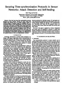
2 Background on Synchronization device 4 3 2 1
t corrupted data (a)
device 4 3 2 1 corrupted data (b)
t
device 4 3 2 1
t (c)
Figure 2.1: Three examples of communication protocols (dotted lines indicate slots, dashed frames). Panel a) depicts the ALOHA protocol, devices transmit data whenever needed. Panel b) depicts the slotted ALOHA protocol. At the beginning of very slot, devices transmit data if needed. Panel c) depicts the TDMA protocol. Devices are assigned to time slots for communication. to transmit a data packet which does not last longer than the time slot, see Figure 2.1b. Data corruption might occur, but due to the time slotting this is a significant improvement to the ALOHA protocol within which every entity can transmit at any point in time, see Figure 2.1a and for example [Gold 05, ch. 14.3]. The protocol does not provide the synchronization process, so for an efficient use of slotted ALOHA, all elements in the system need to be slot synchronized. TDMA The time division multiple access protocol divides the time into time frames and further into time slots. For a transmission a device is assigned a cyclically repeating time slot. It then sends data packets at the assigned slot times, see Figure 2.1c. This protocol provides channel access on a schedule based scheme. This protocol does not provide a synchronization of frames and slots, so for an efficient use, all elements need to be slot synchronized. For a more detailed introduction see for example [Gold 05, ch. 14.2].
2.1.6 Self-Organizing Synchronization Synchronization methods for communication systems were first studied in wired networks. As certain synchronization methods have shown to be reliable they were adapted for use in wireless communication, for example TPSN as an extension of NTP [Serp 09, p. 5]. However this direct transfer of synchronization methods does not exploit the broadcasting nature of wireless systems, i.e. the transmission of any emitted signal to all entities in the emitter’s vicinity. One approach to make use of this effect is by applying self-organizing methods to achieve synchronization. Self-organization is characterized as follows, compare [Dres 07]. • All elements in the system have the same hierarchy. There are no master entities. • All elements in the system perform their local rules. The interplay of all local rules provides a globally emerging behavior.
12
2.2 Networks of Pulse-Coupled Oscillators • The local rules are independent of the number of entities. Therefore, a selforganizing strategy is scalable. • As all entities perform individual local actions, the system is robust to individual drop outs and highly adaptive to small changes. Indeed, research on self-organizing strategies for wireless systems shows these beneficial properties when applying for synchronization [Wern 05, Hong 05, Tyrr 10c, Tyrr 10b, 1, 2]. A basic theory for such strategies is the theory of pulse-coupled oscillators (PCO). It describes an entity via an oscillator and the interactions between them via pulses. In the following section we introduce the theory and show how it relates to synchronization. Later in Section 2.3.3, we give examples of self-organizing synchronization methods for wireless communication systems.
2.2 Networks of Pulse-Coupled Oscillators As a first step we formalize the notion of an oscillator. As a visualization, imagine a typical analogue clock, which only consists of a minute hand. The hand of the clock rotates and repeatedly passes the 12 o’clock sign. We focus on the top of the minute hand and track this point as is moves over time. Since the length of the minute hand does not change, the positions of this top point repeatedly occur and form a circle. For a mathematical model, we neglect the hand of the clock, concentrate on its top point only, and describe its position by a sole parameter, the phase φ, which depends on time t. For simplicity of notation we assume φ(t) to be in the interval [0, 1]. Whenever the oscillator’s phase passes the threshold 1, the phase resets to 0. The point rotates counterclockwise, as this is the mathematical positive rotation for polar coordinates [Bron 07, p. 190]. This is a standard model to describe an individual oscillator and can also be found for example in [Miro 90, Math 96, Timm 02, Timm 04] or in different notation in [Pesk 75, Abbo 93, Vree 94, Vree 96, Erme 96, Erns 95]. As we study a set of N ∈ N oscillators, we use a finite index set I and describe the state of an oscillator i with its phase φi (t). For ease of notation we also use the set I to account for the oscillators themselves. The interactions of an ensemble of oscillators are in the focus of this work. To do so we start by showing an oscillator i’s individual dynamics. In the following sections, we introduce the model assumptions and its notation.
2.2.1 Definition of an Oscillator Let us start with a single fixed oscillator i, which we describe by its phase φi (t) ∈ [0, 1] depending on time t. Its phase rate is defined via dφi φ˙i (t) := = F (φ), dt
(2.1)
where F (·) is a continuous function, mapping [0, 1] into R . Within this thesis we mainly use constant phase rates in particular F (φ) = 1 as in [Miro 90, Timm 02, Nish 11,
13
2 Background on Synchronization PSfrag replacemen φi (t) 1
0 1
p (φ(t)) t
0 (a)
(b)
Figure 2.2: Two representations of the phase evolution. The phase increases linearly until it is reset. Panel a) shows the periodic behavior and the phase jump upon reaching the threshold 1. Panel b) show the a smooth transition of the phase upon reaching the threshold, due to the circular representation via p(φ) as introduced in (2.13).
Nish 12] but also tackle the consequences of different F (·). All F (·) considered provide periodic oscillations, we do not discuss chaotic oscillators. For an introduction on chaotic oscillators see for example [Piko 01, ch. 5]. We denote ci ∈ [0, 1] as the initial condition of oscillator i with ci := φi (0).
(2.2)
Whenever oscillator i reaches the threshold φΘ = 1, it resets, i.e. φi (t) = 1 ⇒ φi (t+ ) = lim φi (t + s) = 0, sց0
(2.3)
and emits a pulse as in [Miro 90, Timm 02, Nish 11, Nish 12, Timm 08], see Figure 2.2a. The pulse emission is also called a firing event. We denote the time corresponding to the nth firing event of the oscillator i with tni .
2.2.2 Pairwise Interaction of Oscillators As we just introduced the emission of pulses, we now consider the reception of such. At a reception event an oscillator immediately adjusts its phase in dependence on its current phase, according to some update function H : [0, 1] 7→ [0, 1]. To be more precise, if an oscillator j receives a pulse from oscillator i at some time tr ∈ R+ := [0, ∞), its phase immediately adjusts with φj (tr ) 7→ φj (t+ r ) = H (φj (tr )) ,
(2.4)
compare [Miro 90, Abbo 93, Vree 94, Erns 95, Vree 96, Erme 96, Math 96, Timm 02, Timm 04, Timm 08, Nish 11, Nish 12]. To simplify notation we address the time instants of a reception event by tr throughout this work. The update function describes the interactions of oscillators. We focus on two types of updates which are called excitatory coupling, see for example [Erns 95], where incoming pulses increase the phases,
14
2.2 Networks of Pulse-Coupled Oscillators φ(t) 1
excitatory inhibitory 0 1
p(φ(t)) 0
tr
tr
0 1
p(φ(t))
t
(a)
(b)
(c)
Figure 2.3: Examples of the two different phase jumps according to the coupling scheme for a) the phase φ and b) and c) the circular representation p(φ) as introduced in (2.13). This demonstrates how the jump can be considered “backward” for inhibitory coupling as in b) and “forward” for excitatory coupling, as in c). as in [Miro 90], see Figure 2.3a, i.e. φj (tr ) < H (φj (tr )) ≤ 1,
(2.5)
and inhibitory coupling [Erns 95], where phases are decreased, as in [Vree 94], i.e. 0 ≤ H (φj (tr )) < φj (tr ).
(2.6)
Depending on the coupling functions qualitatively different types of dynamics may emerge, see Figure 2.4. We also call an excitatory phase adjustment a jump forward and an inhibitory phase adjustment a jump backward, as will be explained in more detail below.
2.2.3 Interaction of an Ensemble of Oscillators The behavior of an individual oscillator and its pairwise interaction, also called the coupling, is described above. For the interplay of several oscillators the overall coupling between the oscillators, also called coupling strategy, needs to be defined. To this end, we use basic notion from graph theory. For an introduction to graph theory see for example [Boll 98]. A node is in relation with another node, if there is an edge that directly links the nodes. The corresponding graph contains all nodes and edges within a network, see Figure 2.5. For our set of oscillators this relates as follows. Interactions within a set I of oscillators are possible if the corresponding oscillators are linked: we identify each oscillator as a node in a graph G(t). At any time t, an oscillator i is linked to another oscillator j, if there is an edge in G(t) from i to j, also called link lij (t). Within the adjacency matrix these edges are stored. If there is an edge or link between i and j, lij (t) = 1, otherwise lij (t) = 0. Note that the graph G(t) is time dependent and can vary over time. This means that links can appear and disappear in the network. However, we assume that the nodes, i.e. the oscillators, remain. By definition, a link is unidirectional, also called directed, i.e. lij 6= lji . We will also consider bidirectional links, also called undirected, i.e. lij = lji . In case of constant
15
φ(t)
1
φ(t)
0 1 0 1 0
φ(t)
φ(t)
φ(t)
φ(t)
2 Background on Synchronization
1 0 1 0 1 0
t (a)
t (b)
Figure 2.4: System dynamics emerging from different coupling schemes. We plot the phase evolution of three oscillators in an all-to-all network and delay-free environment, with random initial conditions. a) We see aligning phases with an update function H(φ) = min(1, 1.1φ). The coupling causes the oscillators to align their phases, as time progresses. b) We see periodic patterns with the update function H(φ) = 0.7φ. Phases adjust to each other but instead of aligning the phases a pattern emerges that causes a periodic phase evolution.
Figure 2.5: Example of a graph G. A set of nodes, represented by dots, is linked via edges, represented via lines.
16
2.2 Networks of Pulse-Coupled Oscillators networks we drop the time dependence in notation. For an oscillator i we define the set of succeeding oscillators by suci (t) := {j ∈ I : lij (t) > 0},
(2.7)
and the set of predecessors by prei (t) := {j ∈ I : lji (t) > 0},
(2.8)
compare [Nish 11]. For a subset S ⊂ I of oscillators and for a point in time t ≥ 0 the set of all predecessors of S is defined by preS (t) := ∪k∈S(t) prek (t),
(2.9)
preS (T ) := ∩t∈T preS (t).
(2.10)
and for a time interval T by
A similar definition applies for sucS (t) and sucS (T ). In case of undirected networks, which is the focus in Chapter 3, we use the term neighboring oscillators which is defined via Ni (t) := {j ∈ I : lij (t) > 0}. (2.11) For an index subset S ⊂ I, we define its edge set via ∂S(t) := {i ∈ S : ∃ j ∈ / S s. t. j ∈ suci (t)}
(2.12)
These are all nodes of S with a link to nodes outside of S. We call two oscillators i and k connected, if there is a path from one to the other, i.e. there are links lij , ljj ′ , . . . , lj ′′ k > 0. If all pairs of nodes in a graph are connected, i.e. every node is connected to every other node, we say that the graph or the network is connected. Within this thesis we study the oscillator dynamics on different kinds of networks, in particular the following. All-to-all network This is a very simple model for a network, every oscillator is linked to every other oscillator. Erd´ os-R˝ enyi random graph (ERG) For an ensemble of oscillators, each link in the network exists with probability plink ∈ (0, 1], see [ErdH 59]. Random geometric graph (RGG) For an ensemble of oscillators, each oscillator is randomly positioned within√the unit square. Two oscillators are linked, if they are within a fixed range r ∈ [0, 2], see [Penr 03].
17
2 Background on Synchronization Arbitrary connected network or meshed network Any network that is connected.
2.2.4 Circular Representation In order to represent the periodic behavior of the phases we also use a circular representation p(φ) of the oscillator phases. We map the phases to a circle of circumference of 1 via � � 1 cos (2πφ(t)) , (2.13) p(φ) : φ(t) 7→ sin (2πφ(t)) 2π see Figure 2.2b, compare [Piko 01]. In this representation, the inhibitory coupling induces a clockwise phase jump and the excitatory coupling a counterclockwise phase jump, see Figure 2.3b and Figure 2.3c.
2.2.5 Delayed Pulses Between the event of an oscillator’s phase passing the firing threshold and the reception of a signal time passes. This time is called the packet delay or simply the delay of a signal [Rhee 09]. It consists of four parts: the sending time, the time needed for a sender to construct the message; the access time, which describes the time until the channel is accessible; the propagation time, the time for a signal to propagate from the sender’s antenna to the receiver’s antenna; and the receive time, which describes the time at the receiver until a signal is decoded [Rhee 09]. Each of these has positive length, and we specifically address delays within this work. Any pulse that is emitted by an oscillator i is subject to some delay τij before it is received at a succeeding oscillator j. This delay might depend on every receiving oscillator and every emission time. To keep track of all pulse emissions in the system, we describe the nth firing event among all oscillators by tn . Note, that this is a notational convention not to be confused with the power operator. As introduced in Section 2.2.3, the links and hence the succeeding oscillators might change over time. Therefore, the transmission process of a pulse needs to be modeled explicitly. We assume that a signal is only going to be received at oscillator j if the corresponding link is available from emission until reception. This yields, � φi (tn ) = 1 ⇒ φj (tn + τijn+ ) = H φj (tn + τijn ) for all j ∈ suci ([tn , tn + τijn ]), (2.14)
compare for example [Gers 96]. For constant networks, suci is constant and we can drop the time dependence. A timeline of these processes is shown in Figure 2.6. Within this work we assume all delays τij are distributed within an interval [τmin , τmax ], 0 ≤ τmin ≤ τmax < 1, with τmin corresponding to the smallest delay and τmax corresponding to the largest delay in the system. We further assume that for every firing event, all delays are uniformly drawn from this interval independently of each other. To emphasize this independence we also use the notation τijn according to every firing event tn .
18
2.2 Networks of Pulse-Coupled Oscillators φ1 (t) 1
0
tr
t
ts′ pulse
φ2 (t)
τ21
τ12
1
0
tr′
ts
t
Figure 2.6: An example of the effect of individual random delays. We plot the phase evolution of two oscillators. At time ts oscillator 2 emits a signal which is received by oscillator 1 with a delay τ21 . The adjustment of oscillator i hence happens at ts + τ21 . Also, the pulse emitted by oscillator 1 at ts′ is delayed by τ12 and received at tr′ . These delayed adjustments can add stochasticity to the system dynamics. Whenever needed, t˜ and t′ represent a time variable (just as t) and τ˜ and τ ′ a delay (just as τ ). The time period between two firing events, also called cycle, of a specific oscillator i is (2.15) − tni . ∆tni := tn+1 i For an isolated oscillator with φ˙ = 1 we hence have ∆tni = 1. In general however, ∆tni can vary with n.
2.2.6 Synchronization of Oscillators We define a distance between two oscillators i and j at time t by dij (t) := min (|φi (t) − φj (t)|, 1 − |φi (t) − φj (t)|) ,
(2.16)
compare [Bron 07, p.150f]. This can be interpreted via the circular representation as the smallest arc between two points on the circle. We further define the precision for a set I of oscillators at some time t via Π(t) := max dij (t), i,j∈I
(2.17)
compare [Kope 03]. Note that in Chapter 3 we need to modify the notion of precision, due to the specific use. In Chapter 4 we again use the definition as introduced here. A general definition would be possible but neither supports a simple notation nor the understanding.
19
2 Background on Synchronization
i dij
p (φ(t)) j
Figure 2.7: An example of the distance as defined in (2.16). The synchronization of oscillators is the process of aligning the oscillator phases. Synchronization is achieved at some time t∗ if Π(t) = 0 for all t ≥ t∗ . The terms being synchronized, in synchrony or in a synchronous state are used equivalently. An ensemble of oscillators is said to be in a close-to-synchrony state, if there is a bound 0 < Γ ≪ 1 and a time t∗ such that Π(t) ≤ Γ for all t ≥ t∗ . Note that the definition of synchrony is inconsistent in the literature. It sometimes corresponds to a close-to-synchrony state, whereas the synchronous state as defined above is referred to as the oscillators being “fully synchronized”, see for example [Olmi 10]. This understanding is often used if full synchrony is not possible, for example due to inhomogeneous phase rates.
2.2.7 Observations on the Synchronization Process The introduction of pulse-coupled oscillators as defined in Section 2.2 leads to some immediate observations: • The instantaneous updates cause nonlinear and discontinuous dynamics. • The individual and random delays at the signal transmission induce stochastic effects. • The connectivity of the underlying network may change non-deterministically. As it directly influences the dynamics this induces further randomness to the system. • A general synchronization statement needs to be independent of the stochastic effects and underlying topology and has to hold for all initial conditions (2.2). For these reasons differential equations do not provide a suitable description of this system. Hence we use an event based approach to study the system dynamics. One idea using such an approach is to transfer the synchronization problem to a fixed point problem, as done by Mirollo and Strogatz e.g. in [Miro 90]. For a detailed introduction to the fixed point theorem see for example [Rudi 76].
2.2.8 Other Applications of Pulse-Coupled Oscillators The theory of pulse-coupled oscillators is a mathematical concept which can be used to describe phenomena in different fields of research. It is being used to describe the
20
2.2 Networks of Pulse-Coupled Oscillators phenomena of synchronization and thereby serves as a model for self-organization. We describe a few examples for illustration. Zoology The flashing rhythm of fireflies in South East Asia is considered a prime example of a self-organizing synchronization phenomenon [Stro 03, Dres 07]. Thousand of fireflies gather in trees at dawn and start to emit short light signals with some intrinsic frequency. As the fireflies communicate their blinking, some species align their blinking and end up in a synchronized flashing behavior. Even though scientists tried to explain the phenomenon, it was not before the second half of the last century that the idea of a self-organizing approach was anticipated, and indicated via experiments [Winf 67, Hans 71, Buck 81, Cama 01]. In order to understand how synchronization emerges, fireflies were described as oscillators and mathematical models for the dynamics of these oscillators were introduced [Winf 67, Hans 71, Buck 81, Cama 01]. Winfree [Winf 67] and Kuramoto [Kura 75] studied continuous-coupled oscillator systems, whereas Peskin [Pesk 75] introduced a pulse-coupled oscillator system which appeared to be more suitable for the discrete coupling. Interestingly, Peskin’s model originally stems from describing pacemaker cells for the heart. Peskin could show that synchrony emerges for two oscillators, under very restricted assumptions. Guided by this insight he postulated that also arbitrarily large sets of oscillators would eventually synchronize [Pesk 75, Stro 93]. Mathematics As pulse-coupled oscillators were subject to mathematical analysis, the non-linearity and discontinuity induced by the pulse-coupling showed to complicate the understanding of the underlying dynamics. It was relatively easy to understand the dynamics for two oscillators, but analytical generalization was not achieved until 1990. That is when Mirollo and Strogatz showed that starting from almost all initial conditions any set of oscillators, for certain idealized system assumptions, eventually ends up in synchrony [Miro 90]. Two considerations were essential for this proof. First, they studied a discretized version, which means they only consider the system state at discrete times, when a specific oscillator fires. In mathematical terms, these are called Poincar´e maps, see for example [Guck 02]. Second, they identified dynamics within these discrete maps and demonstrated that the phases converge to the fixed point of full synchrony. This is the case for almost all initial conditions. Their work gave significant insight into self-organizing synchronization. However, their result was bound to some simplifications and restrictions. They assumed that all oscillators were connected to all other oscillators, that any pulse was received infinitesimally short after emission, and that all oscillators have an identical and homogeneous phase rate. Additionally, their proof only holds for a certain class of update functions and excitatory coupling. Excitatory coupling is indeed the strategy for synchronization within some types of fireflies. Others, however, use a combination of excitatory and inhibitory
21
2 Background on Synchronization coupling for this goal [Cama 01]. Interestingly, further research on synchronization tended to focus on excitatory coupling [Math 96, Hong 05, Tyrr 10b, Pagl 11], potentially through the influence of the seminar work of Mirollo and Strogatz. Still, specific synchronization statements using inhibitory coupling can be made [Vree 94, Timm 02], [1]. But it was not until recently that interest and results on synchronization were achieved using a combination of inhibitory and excitatory coupling [Nish 11, Nish 12, Wang 12], [2]. Neuroscience The pulse-coupling oscillator model is also used to study pacemaker networks at the heart or neuronal activities in the brain [Pesk 75, Brun 99]. Neurons are electrically excitable cells that emit electrical signals, called spikes, and react to electrical signals. Neuroscientists and physicists are interested in emerging firing patterns as they are believed to be related to how the brain processes information and learns [Hint 92]. At the same time synchronization is not always desirable, as the formation of synchronization of neural dynamics may cause epileptic seizure [Neto 04]. As the theory of pulse-coupled oscillators is studied in neuroscience great insight on certain dynamical effect was gained. However, this insight is often not directly applicable for synchronization processes in wireless communication systems as the theoretical system assumptions differ just like the research focus. Some areas of the brain consist of excitatory neurons, or inhibitory neurons or a combination of both. This steered research in different directions such as studying the interactions of purely inhibitory coupled oscillators. It appears that inhibitory coupling can better provide synchrony under certain conditions, such as the presence of positive transmission delays [Vree 94, Erns 95, Vree 96, Erns 98]. For example if all oscillators emit a signal before the first receives one, global synchrony can be achieved [Timm 02]. Since neurons typically do not form all-to-all networks, the study of synchronization within sparsely or not all-to-all networks was prevalent. This brought great insight in terms of stable periodic patterns and the influence of inhibitory coupling on stability [Memm 10, Erns 98]. Also other effects such as the interplay of excitatory and inhibitory neurons [Golo 01], or the aspect of unreliable links [Kinz 08], which is of specific interest in Chapter 4, are studied.
2.3 Synchronization of Pulse-Coupled Oscillators Research on synchronization of pulse-coupled oscillators started with idealized assumptions such as oscillators with interactions on an all-to-all network, also called all-to-all coupling and delay-free environments. Within this section we explain and give examples how the dynamics within a PCO system changes if the system confronts delays and not all-to-all coupling. These generalizations increase the complexity of the system and synchronization not necessarily emerges. This causes researchers to either change the oscillator interactions such that a close-to-synchrony state still emerges or to focus on more specific system dynamics without aiming at synchronizing the system.
22
2.3 Synchronization of Pulse-Coupled Oscillators
Table 2.1: Phase evolution Example 1. t t1 t1+ t2 t2+ t1 + τ t1 + τ + t2 + τ t2 + τ +
of oscillators 1 and 2, and precision Π from (2.17) as in φ1 1 0 ε ε τ τ ε+τ α(ε + τ )
φ2 1−ε 1−ε 1 0 τ −ε α (τ − ε) α(τ − ε) + ε α(τ − ε) + ε
Π(t) ε ε ε ε ε τ − α(τ − ε) τ − α(τ − ε) (2α − 1)ε
2.3.1 Generalizations on Delays Early generalizations for pulse-coupled oscillator systems concentrated on delayed pulses [Kura 91, Erns 95, Erns 98, Math 96, Gers 96]. Researchers addressed both constant homogeneous delays as well as variably changing delays within some delay window. In any case it turned out that as soon as signals are not received immediately after emission the synchronous state does not emerge [Kura 91, Erns 95, Gers 96]. Moreover, even if the system is initially in the synchronized state, small fluctuations due to noise lead to a break up of the synchronized state [Erns 95, Erns 98]. Consider a system of two oscillators, which are very close to synchrony, and constant delays. Assume both emit a signal and later on both adjust. The situation arises, that when adjusting, both oscillators react to pulses from the past, but now, after resetting, with a totally different phase. This can drive close oscillators further apart and thereby hinder synchrony, see Example 1. Example 1. Let us take a set of oscillators {1, 2}, identical phase rates, all-to-all coupling, and an update function H(φ) = min(1, αφ) with α > 1, and constant pulse delays with τ = 0.1. Let us further assume φ1 (t1 ) = 1, and φ2 (t1 ) = 1 − ε, 0 < ε < τ , hence the precision Π(t1 ) = ε. Oscillator 1 fires and resets at t1 , so does oscillator 2 at t2 . At reception time t1 + τ , we have φ1 (t1 + τ ) = τ , φ2 (t1 + τ ) = τ − ε and thus φ2 (t1 + τ + ) = α(τ − ε). At t2 + τ we have φ1 (t2 + τ ) = ε + τ with φ1 (t2 + τ + ) = α(ε + τ ) and φ2 (t2 + τ ) = α(τ − ε) + ε, see Table 2.1. Hence Π(t2 + τ + ) = (2α − 1)ε > ε = Π(t1 ), and the phase difference of the oscillators increases. If the delays are not even homogeneous, two coinciding oscillators emit pulses at the same time but receive the corresponding pulse from the other oscillator at different times. The reception causes each oscillator to adjust and thereby synchrony is lost, see Example 2. This situation could not occur if there were no delays, since then the resetting would precede the adjustment. Example 2. Consider two oscillators indexed by {1, 2} with identical phase rates, allto-all coupling, and an update function H(φ) = min(1, αφ) with α > 1, and individual
23
2 Background on Synchronization
Table 2.2: Phase evolution of oscillators 1, 2 and the precision Π from (2.17) as in Example 2. t φ1 φ2 Π(t) t1 1 1 0 t1+ 0 0 0 1 t + τ12 τ12 τ12 0 + 1 t + τ12 τ12 ατ12 α(1 − τ12 ) 1 t + τ21 τ21 ατ12 + τ21 − τ12 α(1 − τ12 ) + t1 + τ21 ατ21 ατ12 + τ21 − τ12 (τ21 − τ12 ) (α − 1) pulse delays with τ12 < τ21 . Assume that the oscillators are synchronized with φ1 (t1 ) = + φ2 (t1 ) = 1, which yields the precision Π(t1 ) = 0. They both fire and reset, hence φ2 (τ12 )= + ατ12 and φ1 (τ21 ) = ατ21 and consequently Π(t1 + τ21 ) = |ατ12 + τ21 − τ12 − ατ21 | = (α − 1)(τ21 − τ12 ) > 0, and synchrony is lost, see Table 2.2. In order to overcome this effect, Kuramoto introduced a refractory period φref [Kura 91], also called refractory interval, every time an oscillator emitted a pulse. As a consequence, oscillators that just fired enter a phase interval within which no adjustments are done, i.e. + φi (t0 ) = 0 φj (t0 + τij+ ) = φj (t0 + τij ) if φj ≤ φref ∀j 6= i . (2.18) φi (t0 ) = 1 ⇒ φj (t0 + τij+ ) = H (φj (tn + τij )) if φj > φref ∀j 6= i The desynchronization illustrated in Example 2 depends on the delays. The refractory interval mitigates small delays and simulation results indicate that for any initial condition the close-to-synchrony state is achieved [Math 96]. Adding a delay to pulse-coupled oscillator systems changes the dynamics fundamentally. The fully synchronous state is not achievable anymore [Lund 84], as a consequence of τ > 0. The firing order of the oscillators does not necessarily stay constant, as a consequence of τij 6= τik . The individually changing delays introduce a stochastic process and can change the index sequence of firing oscillators. Hence the total dynamics cannot be studied via repeating index sequences as it was done for example by Mirollo and Strogatz [Miro 90]. Here is an example of such a twist in firing sequence.
Example 3. Consider a set of three oscillators indexed by {1, 2, 3} and all-to-all coupling. Let oscillator 1 fire at t1 and the index sequence of firing oscillators is the repeating tupel (1, 2, 3). So the next oscillator to fire would be oscillator 2, hence φ2 (t1 ) > φ3 (t1 ). Oscillator 1 emits a signal to the other oscillators with the delays 0 < τ12 ≪ 1 and 0 < τ13 ≪ 1. If τ13 < τ12 and excitatory phase adjustments, it is possible that with + + ). Hence the new index ) > φ2 (t1 + τmax 0 < φ2 (t1 ) − φ3 (t1 ) ≪ 1 we have φ3 (t1 + τmax sequence of firing is (3, 2, 1) which is equivalent to (1, 3, 2) and differs from the original, see Table 2.3.
24
2.3 Synchronization of Pulse-Coupled Oscillators
Table 2.3: Phase evolution and phase ordering of oscillators 1, 2 and 3 as in Example 3. t φ1 φ2 φ3 φ2 vs. φ3 1 t 1 c2 c3 > t1+ 0 c2 c3 > t1 + τ13 τ13 c2 + τ13 c3 + τ13 > + t1 + τ13 τ13 c2 + τ13 H(c3 + τ13 ) > t1 + τ12 τ21 c2 + τ12 H(c3 + τ13 ) + τ21 − τ13 > + 1 t + τ12 τ21 H(c2 + τ12 ) H(c3 + τ13 ) + τ21 − τ13 < Summarizing, delays can have negative effects on the synchronization of such pulsecoupled systems. In order to still provide synchronized systems or close-to-synchrony states in systems, researchers modify the coupling between the oscillators. This search for appropriate coupling hence became an engineering task. Even though researchers introduced new specific coupling strategies combining both inhibitory and excitatory coupling with sole focus on wireless communication applications [Nish 11, Nish 12, Wang 12, Naka 12], [1] this coupling concept is known to also exist in nature [Buck 81, Erme 96].
2.3.2 Synchronization in Arbitrary Connected Networks In order to synchronize, information has to be communicated through the network. From an analytical perspective, it is much easier to study synchronizing dynamics on all-to-all networks than on arbitrary connected networks. This is not surprising, as an all-toall network provides far more homogeneous dynamics compared to arbitrary connected networks. Also the variety of networks is much larger for arbitrary connected networks, therefore it is also much more difficult to obtain a synchronization statement that is valid on all of these. For specific situations statements were made: For example, Timme et al. predict the speed of convergence and shows that there is speed limit for inhibitory coupled systems on random networks. This limit depends on the pulse-coupling and the topology [Timm 04]. Nishimura and Friedman show the emergence of synchrony for as the network size goes to infinity [Nish 12]. Memmesheimer and Timme showed that by designing the network structure certain dynamics are achievable [Memm 06], which seams to be a promising start.
2.3.3 Self-Organizing Synchronization for Wireless Communications Synchronization of pulse-coupled oscillators is a self-organizing process. As self-organizing methods are also appealing in wireless communication systems, see Section 2.1.6, researchers tried to apply the theoretical model to more realistic environments [Math 96, Wern 05, Hong 05, Tyrr 06, Tyrr 10c, Tyrr 10b],[1, 2]. Whereas simulations and numerical results could draw a promising picture about realizations, actual implementations encountered further difficulties, see for example [Wern 05, Tyrr 10b]. The most prevalent difficulty is the notion of a pulse. Whereas a pulse is an abstract concept as the Dirac R∞ distribution δ(t) which is defined by −∞ δ(t)dt = 1 and δ(t) = 0, ∀t 6= 0, it cannot be 25
2 Background on Synchronization realized, compare [Tyrr 10b]. As an approximation of a pulse, a unique signal is used in wireless communications. This signal is called a beacon or a sync-word. All entities within a system use this beacon, which has non-zero length, to communicate the pulse. By doing so two drawbacks arise. On the one hand the positive length creates an additional pulse delay. Since the devices exchange data additionally to the beacon, a device has to differentiate if an incoming signal is a beacon or some data. This creates an additional delay, since it takes the device time to make this decision. On the other hand a beacon with positive length can get corrupted, just like any data can get corrupted if several devices send data which interfere with each other. The probability for this to happen might be small for small networks, but the larger the network the more likely this becomes and eventually scalability has its limits. Let us discuss two methods that cope with these limitations by transmitting time stamps or exchanging pulse-like signals. Exchanging Time Stamps One way is to send a beacon and append some additional information such as a time stamp. Whenever such a signal is picked up, the receiver can extract the emission time of the beacon and, by using this emission time to process, the beacon can be considered almost as a delay free signal [Dali 03, Wern 05, Leid 10]. By using such a time stamp the algorithm is very close to the idealized environment, which might allow a better reasoning to apply the convergence proof of Mirollo and Strogatz [Miro 90]. Additionally, some identification of the emitter can be attached and every oscillator can decide if it trusts the emitter or not. As a consequence a robust system is created that can - to some extent - cope with erroneous elements [Dali 03, Wern 05]. As a disadvantage, such a system is no more using pulses, which means, that one of the characteristics of pulse-coupling, the sending of as little information as possible, is lost. Additionally, the appending of data to the pulse-like-signal increases the whole signal length, and thereby increases the probability of inferences and reduces the scalability advantages. Exchanging Pulse-like Signals The second method is to use a pulse-like-signal, i.e. a beacon, and a specific correlator to detect the beacon. A receiver senses the channel, receives data and at the same time correlates it with the beacon. So even if data is corrupted, there is a rather high probability that the correlator can detect that within the corrupted data a beacon is buried [Tyrr 10b]. This strategy allows a smooth transition of the pulse-coupled oscillator theory to wireless environments, with all its advantages as described in Section 2.1.6. On the down sides, additional hardware is needed, the correlator, which is not standard for a wireless communication device. Additionally, the probability to detect such a pulse is large but not 1, which the theory has to account for. The finite length of the beacon also has it that a device needs time to emit the signal. Since standard wireless devices only have one unit for transmitting and receiving, called a transceiver, they cannot adjust while sending. This is called the half-duplex constraint.
26
2.3 Synchronization of Pulse-Coupled Oscillators MEMFIS receive mode Every nodes changes mode due to stochastic process
φref r 0 listen
MEMFIS transmit mode
data sync word
0 data
Figure 2.8: The two possible modes of an oscillator within the MEMFIS algorithm. The modes change due to a scheduling process. Any device in the receive mode listens to the channel and upon receiving a signal, adjusts its phase unless in refractory period. Any device in the transmit mode sends data and includes the pulse-like sync-word. We give an overview of two synchronization protocols that use pulse-like signals. MEMFIS The MEMFIS algorithm [Tyrr 10b] is a way to incorporate the synchronization process into a packet transmitting procedure. It performs an excitatory coupled synchronization procedure based on the Mirollo and Strogatz model, additionally using a refractory period. It uses a beacon, also called sync-word, instead of a pulse, copes with timevarying delays, and incorporates two modes, a transmitting and a receiving mode to overcome the inability of simultaneous sending and receiving. Whenever a data packet is to be sent, the beacon is included in the packet. This imposes a probabilistic synchronization process, since data packets are issued by another application layer of an entity and therefore follow some arrival distribution. All entities in the system that are not assigned a transmission are in the receive mode. These entities adjust to the incoming beacon. The basic outline can be seen in Figure 2.8, where the phase of an oscillator is mapped onto a circle and the state of an oscillator is divided into the receive mode and the transmit mode. Within the receive mode a device listens to the channel and adjusts upon receiving a signal unless it is in the refractory period φref . This period represents the deafness interval within which no adjustments are performed. In the transmit mode the data transmission and the incorporated sync-word transmission is performed. PCO Protocol The pulse-coupled oscillator protocol (PCO protocol) [Pagl 11] also uses pulse-like signals for synchronization and combines this process with communication. To overcome system restrictions beacons are used instead of pulses, a refractory period is used to overcome negative effects due to noise. Devices switch their transceivers to transmission when about to fire and to receive otherwise. Potential negative synchronization effects caused by switching are hindered by the use of a refractory time. In order to include data communication two different modes are used. First within the “PCO bootstrap” mode, no data except the beacons are exchanged. Synchronization takes place within this mode. After a fixed amount of cycles the devices switch to the
27
2 Background on Synchronization PCO maintenance mode
PCO bootstrap mode
some nodes perform:
most nodes perform:
All modes change mode at some point φref r transmit 0 listen
φref r transmit
data data 0
listen
Figure 2.9: The two possible modes within the PCO protocol. After the PCO bootstrap mode, all devices switch to the PCO maintenance mode. “PCO maintenance” mode. This transition from one mode to the other can also be done gradually. Within the second mode a large number of entities and cycles is used for data communication, see Figure 2.9.
2.4 Design Principles for Self-Organizing Synchronization The theory of pulse-coupled oscillators can be used to design self-organizing synchronization methods for wireless communication applications. Distributed devices exhibit local actions and enable a global effect, the emergence of synchronization. The transition of the theory from idealized assumptions to wireless communication systems however can cease this emergence as shown in Section 2.3.1. Still, a guaranteed synchronization within wireless communication systems is needed to actually use this self-organizing synchronization approach for communication standards, such as the IEEE (Institute of Electrical and Electronics Engineers) wireless communication standards, see for example [Gold 05, p.23f]. This thesis addresses this need by providing synchronization schemes that guarantee to synchronize an ensemble of pulse-coupled oscillators. Including these schemes in existing self-organizing synchronization methods such as the MEMFIS algorithm, see Section 2.3.3, wireless communication systems are then guaranteed to synchronize. This design approach is described in more detail in the following.
2.4.1 Modeling Approach As a first step, we use the pulse-coupled oscillator theory and introduce general system assumptions in order to address the wireless communication systems. We design the pairwise interactions between oscillators such that synchronization is achieved. By analytical proofs we guarantee that synchronization emerges. In a second step, for a given wireless communication system with the need for synchronization, we apply the synchronization scheme with the appropriate system assumptions and intentionally design the coupling of the entities. As a third step, we incorporate the synchronization scheme into existing communication protocols. By doing so, we rely on work from the literature for the actual realization,
28
2.4 Design Principles for Self-Organizing Synchronization but are able to guarantee that the realization synchronizes the wireless communication systems, as long as our system assumptions are met.
2.4.2 Designing Update Functions for Synchronization As the system assumptions should be as general as possible, the only way to change the dynamics of the system is by designing the update function which describes the pairwise interaction between oscillators and hence the coupling. We use two different approaches to design the update function. Inhibitory Coupling Guided by the synchronization statements from Timme et al. [Timm 02] we design a coupling strategy which uses inhibitory coupling. For all-to-all pulse-coupled oscillator systems with phase rate inhomogeneities and individual random delays, we prove that synchronization emerges, see Chapter 3. Inhibitory and Excitatory Coupling Work regarding the design and use of a combination of inhibitory and excitatory coupling can be found in the literature. Wang et al. [Wang 12] showed that an update function that incorporates both inhibitory and excitatory coupling can improve the time to synchronize. Nakada and Miura [Naka 12] revealed similar results for large delays. Nishimura and Friedman showed that the fully synchronized state is stable if coupling includes both inhibitory and excitatory coupling [Nish 11]. They further extended their work and showed that for as the network size goes to infinity synchrony almost always emerges for all initial conditions [Nish 12]. Nevertheless a coupling strategy that provides synchronization on arbitrary networks, independent of the initial condition was not available. We extend the work on inhibitory and excitatory coupling by additionally introducing stochastic pulse emission. For the so designed coupling we prove that all systems of pulse-coupled oscillators synchronize for all initial conditions. We give a motivation and detailed proof in Chapter 4.
2.4.3 Synchronization Strategies Depending on how the system assumptions are formed, different coupling schemes are needed to provide synchronization. This characterizes our approach in Chapter 3 and Chapter 4. Each chapter, independently of each other, provides a synchronization strategy for specific system assumptions. It gives a self-contained picture and also marks the limits of application. Within each chapter we first introduce the specific system assumptions and then give specific coupling rules such that synchronization is emerging. We prove that the specific coupling is guaranteed to emerge and elaborate on the system’s dynamics regarding synchronization time and robustness. In Chapter 5 we show
29
2 Background on Synchronization implementations of the coupling strategies and elaborate on the applicability and its limitations.
30
3 Synchronization with Inhibitory Coupling Within this chapter we introduce an inhibitory coupling scheme that synchronizes pulsecoupled oscillator systems started from arbitrary initial conditions, and independent of the number of oscillators. This coupling scheme is proven to synchronizing using the following assumptions • all-to-all network, • arbitrary initial condition, • arbitrary number of oscillators, • random individual delays, • heterogeneous phase rates. In case of homogeneous phase rates and a delay-free system, we guarantee full synchrony. For heterogeneous phase rates and random individual delays a close-to-synchrony state is reached. The results presented in this chapter have been achieved in cooperation with Christian Bettstetter and Marc Timme and are published in [1, 6, 4]. Parts of this chapter are taken from [1]. The following observation was the key motivation for the use of inhibitory coupling for synchronization.
3.1 Motivation 3.1.1 Beneficial Synchronizing Effects For the design of an update function we first show two examples which demonstrate some dynamics caused by inhibitory coupling. Example 4. Let us assume a set of oscillators {1, 2, 3}, a delay-free system, homogeneous phase rates, an all-to-all network and the update function H(φ) = (1 + α)φ. At some time t1 oscillator 1 fires and emits a pulse to oscillators 2 and 3. We define φ2 (t1 ) = c2 and φ3 (t1 ) = c3 . After pulse reception we have φ2 (t1+ ) = (1 + α)c2 and φ3 (t1+ ) = (1+α)c3 . Hence |φ2 (t1+ )−φ3 (t1+ )| = |(1+α)c2 −(1+α)c3 | = (1+α)|c2 −c3 | = (1 + α)|φ2 (t1 ) − φ3 (t1 )|. Therefore the difference between the two oscillators increases if α > 0, which is an excitatory coupling, and decreases if α < 0, which is an inhibitory coupling.
31
3 Synchronization with Inhibitory Coupling We see that in Example 4 inhibitory coupling decreases the phase difference of the receiving oscillators. This is a positive effect for synchronizing dynamics and can contribute to the robustness of the synchronization process. Additionally, inhibitory coupling can keep up the oscillators’ order, as can be seen in the following example. Example 5. Let us assume a set of oscillators I = {1, 2, 3, . . . , 10}, a delay-free system, homogeneous phase rates, an all-to-all network and the update function H(φ) = (1+α)φ, with −1 < α < 0. Further let us assume that at time t1 we have φ10 (t1 ) = 1 and the oscillators are in ascending order such that φi (t1 ) ≤ φi+1 (t1 ), for i ∈ {1, . . . , 9} and define φi (t1 ) = ci for all i. Oscillator 10 fires and resets and emits a pulse to all other oscillators. These adjust and we have φi (t1+ ) = (1+α)ci for all i ∈ I \{10}. We observe that for all i ∈ I \ {9, 10} we have (1 + α)ci ≤ (1 + α)ci+1 , and thus the firing event did not change the order of the oscillators {1, . . . , 9}. The example shows a very interesting property for this inhibitory coupled network. The order of the oscillators does not change for all not-firing oscillators. In both examples the firing oscillator does not provide the properties which are beneficial for synchronization and causes inhomogeneities. Since we intend to design a synchronization scheme and apply the algorithm to a wireless communication system, we modify the resetting behavior. We simply define that an oscillator upon firing, does not reset. Instead, it inhibitorily updates its own phase as if the pulse was from another oscillator, i.e. it self-adjusts. This introduction of self-adjustment totally changes the dynamics of the system. We see that if we demand self-adjustment for the firing oscillator, the Example 4 and Example 5 both provide homogeneous behavior. To be more precise, the phase difference of all oscillators decreases compare Example 4 and also the order of all oscillators is kept after a firing event, compare Example 5.
3.1.2 Outline of the Proof This minor change in coupling scheme shows to have great effects on the synchronization behavior. Here is a rough overview of these two effects for delay-free, all-to-all coupled systems with homogeneous phase rates, as shown in the examples above. If all elements in the system adjust to a pulse, all phase differences decrease. This holds for every pulse emission and provides a monotonically decreasing precision. As the precision is bounded by zero from below, the phase differences converge to zero. Example 4 even indicates an exponential decay. The second effect, the conservation of the firing order, simplifies the modalities for the proof. As the order of oscillators does not change, the oscillator that fires first, will continue to stay in the lead. Hence this oscillator repeatedly fires and oscillators with lower phase will never fire. As a consequence we can focus on the firing events of the first oscillator and consider these as a strictly decreasing sequence. These effects are the core arguments for the proof on synchronization. As we will see in the following, we can even relax the system assumptions up to those given in the beginning of this chapter and still prove synchronization. This generalization, however,
32
3.2 Specifying the System Settings causes a lot of technical specifications and distinction of cases. In order to still keep the line of arguments easy to follow, we start with a convergence statement for two oscillators. This provides all necessary steps and argumentation principles needed for an ensemble of oscillators, which leads to the main synchronization theorem in this chapter.
3.2 Specifying the System Settings The general system setting is defined in Section 2.2, which introduces the pulse-coupled oscillators. As explained in Section 2.4.3, we need to individually specify the systems settings in order to give synchronization statements. Here is a compact description of the system assumptions used in this chapter.
3.2.1 Oscillator Properties We use a set I of N oscillators. Concerning their phase rates, compare (2.1), we assume constant but possibly different phase rates. Hence, for the phase rate of oscillator i we have dφi (t) := φ˙i (t) := κi with κi ∈ [1 − ν, 1 + ν], 0 ≤ ν ≪ 1, (3.1) dt where ν is the maximum phase rate deviation. For the further analysis we consider small deviations only. Let us assume an all-to-all network, i.e. Ni = I \ i for all i ∈ I, and individual random pulse delays within a delay window [τmin , τmax ]. We assume 1 τmax < 1+ν (1 − H(1)).
3.2.2 Oscillator Coupling We introduce the self-adjustment, such that also the firing oscillator adjusts to its fire instead of resetting. Hence at a firing event of oscillator i at time tn we have � φi (tn+ ) = H (φj (tn )) n φi (t ) = 1 ⇒ . (3.2) φj (tn + τij+ ) = H (φj (tn + τij )) ∀j 6= i For the update function H(·) we assume a twice continuously differentiable function 2 with H(0) = 0, 0 ≤ H(φ) ≤ 1 and d H(φ) ≤ 0 for all phase values φ(t) ∈ [0, 1]. We define dt dH(φ) ′ ′ ′ ′ = minφ H ′ (φ). We show an example of H (φ) = dφ , Hmax = maxφ H (φ) and Hmin such a function in Figure 3.1a. Following this update function, upon pulse reception, an oscillator always performs non-positive phase jumps, i.e. the system is inhibitorily coupled. Due to this modification, the phase interval of an isolated oscillator is now [H(1), 1] after the first firing event. The interactions of two coupled oscillators i and j can be seen in Figure 3.1b. Oscillator i reaches the threshold, fires, and performs a phase jump to H(1). After some delay τij , oscillator j receives the fire pulse and adjusts its phase as well. It jump to a phase lower than H(1). As both oscillators again increase their phases, oscillator i fires again, and the adjustments repeat.
33
3 Synchronization with Inhibitory Coupling H(φ) φ(t) 1
1
τ
τ′
H(1) 0
1
φ
(a) Example of an update function H(·).
0
t1
t2
t
(b) Phase evolution of two oscillators using inhibitory coupling.
Figure 3.1: Update function and phase evolution with inhibitory coupling and selfadjustment. Algorithm 1 Synchronization with inhibitory coupling and self-adjustment. 1. An oscillator i increases its phase φi from 0 to 1 (∀ i ∈ I). 2. Whenever an oscillator i reaches φi (t) = 1, the oscillator sends a pulse and adjusts its phase to φi (t+ ) = H(1) (instantaneous self-coupling). 3. The refractory interval is φref = H(1) + 2(1 + ν)τmax . 4. Whenever an oscillator j receives a pulse from i (reception time t+τij ): a) It adjusts its phase to φj (t+τij+ ) = H(φj (t+τij )) if φj (t+τij ) ∈ / [0, φref ] (∀j 6= i).
b) It keeps its phase at φj (t+τij+ ) = φj (t+τij ) if φj (t+τij ) ∈ [0, φref ] (∀j 6= i).
3.2.3 Refractory Interval In order to overcome negative coupling effects as described in Example 1 and Example 2 we use a refractory interval, compare (2.18). Without a refractory interval, synchronized oscillators can adjust to each others pulses due to different propagation delays, see Example 2, this is called an echoing effect. The refractory interval is constructed such that any oscillator phase does not experience these echoing effects. To do so, the cycle interval of an isolated oscillator, which is [H(1), 1] after the first firing event, has to be taken into account. The same applies for the maximum delay τmax , and the maximum possible phase rate 1 + ν. Consequently, at a firing time tn , the refractory interval is set to [0, φref ] with φref = max {φi (tn + 2τmax )} = H(1) + 2(1 + ν)τmax . i∈I
(3.3)
All oscillators with their phases in this interval do not adjust upon reception of a pulse. The entire synchronization scheme is summarized in Algorithm 1 and denoted as synchronization with inhibitory coupling and self-adjustment (SISA).
34
3.2 Specifying the System Settings tn :
tn+ :
0 1
H(1)
p(φ) (a)
0 1
H(1)
p(φ) (b)
0 1
H(1)
p(φ) (c)
Figure 3.2: Circular phase representation, using p(φ) from (2.13), with inhibitory coupling as defined in (3.2) and (3.3). The dark dot represents the phase position of the firing oscillator. Panel a) visualizes the phase jumps of a firing oscillator and an adjusting oscillator. Panel b) shows an example of an ensemble of oscillators at a firing event at time tn . Panel c) illustrates the phase positions of the example from panel b) right after the phase adjustments at tn+ in a delay-free system.
3.2.4 Alternative Circular Representation Using the circular phase representation from (2.13), the system dynamics of the coupling from (3.2) and (3.3) can be shown on a circle. Upon a firing event the firing oscillator self-adjusts. Upon a reception event an adjusting oscillator jumps backward on the circle. An example is given in Figure 3.2a. The main idea of the circular representation is to have a smooth phase representation of a firing oscillator, in particular when the firing oscillator resets. With the phase representation from (2.13), this is not the case, as visualized in Figure 3.2a. To still provide such a smooth phase evolution we introduce an alternative circular representation p˜ : [0, 1] 7→ [0, ω), with ω = 1 − H(1). We account for the phase interval for an isolated oscillator, which is [H(1), 1] and cycle length ω, and provide a smooth phase representation. We define � l(φ) := φ − H(1) mod ω, (3.4) and the alternative circular representation via � � l(φ) . p˜(φ) := p ω
(3.5)
This representation brings a smooth transition for the self-adjustment,see Figure 3.3a. It is also applicable for an ensemble of oscillators, see Figure 3.3b and Figure 3.3c. We will need this representation later on in Section 3.7. For the adjusting oscillators this representation brings a new interpretation of the coupling scheme. Via p˜(φ) the adjusting oscillators (disregarding the self-adjusting ones) can be considered as performing a positive phase jump see Figure 3.3b and Figure 3.3c. However, the phase of such an adjusting oscillator j after adjustment at time tr is φj (t+ r ) < H(1) and hence it does not fire when passing the p˜(φj ) = ω threshold.
35
3 Synchronization with Inhibitory Coupling tn+ :
tn : 0
0
0
ω
ω
ω
p˜(φ) (a)
p˜(φ) (b)
p˜(φ) (c)
Figure 3.3: Alternative circular representation using p˜(φ) from (3.5). The dark dot represents the phase position of the firing oscillator. Panel a) shows the smooth transition of the firing oscillator upon self-adjustment. Panel b) depicts an example for an ensemble of oscillators at a firing event at time tn . Panel c) illustrates the phase positions right after the adjustments at time tn+ for a delay-free system.
3.2.5 Leading Oscillator Let us define an index permutation γi , i ∈ {1, . . . , |S|}, such that p˜(φγi ) ≤ p˜(φγi+1 ) for all i. In other words, we position the oscillators on a circle of circumference ω, and denote them in ascending order of their phases, see Figure 3.4. Then oscillator i∗ with ( φγi+1 − φγi for i < N , (3.6) i∗ := arg max i=1,...,|S| 1 − φγ + φγ for i = N 1 i is called the leading oscillator or leader. Figuratively speaking, this is the oscillator that starts the pulse emission for the set of oscillators for a cycle, for examples see the dark dot in Figure 3.2b, Figure 3.2c, Figure 3.3b and Figure 3.3c. This definition of the leading oscillator is only valid for any time after the first firing event. The leading oscillator is used to characterize a cycle for the whole set of oscillators. This leading oscillator might change over time due to the different phase rates and due to the initial conditions. However, as soon as the fastest oscillator is in the lead, it will stay in the lead, as we will see in Lemma 3. The firing time of the leading oscillator in the nth cycle is denoted by tn◦ .
3.2.6 Sample Synchronization Process By visualizing a sample synchronization process we identify the key argument for the convergence statements. A set of oscillators starts from random initial conditions in a delay-free system with homogeneous phase rates and coupled as defined in (3.2) and (3.3), see Figure 3.5. With every firing event the oscillators move closer together. Additionally, we see the advantage of introducing (3.5), as the contracting property within the system becomes more visible. In Figure 3.6 the corresponding alternative circular representation p˜(φ) is shown. This also demonstrates how the introduces alternative circular representation can be used to visualize the contracting dynamics of the system.
36
3.2 Specifying the System Settings
γ3
γ2 γ1 0 ω
γ4 γ5 γ 6 = i∗ p˜(φ)
Figure 3.4: The index permutation of the oscillators. According to the alternative circular representation p˜(φ) from (3.5) the oscillators are denoted in ascending order. The oscillator at the largest arc is denoted by i∗ , as in (3.6).
φi (tn )
1 0.5
l (φi (tn ))
0
t1
t1+
t2
t2+
t3
t3+ n
t4
t4+
t5
t5+
t6
t6+
t1
t1+
t2
t2+
t3
t3+ n
t4
t4+
t5
t5+
t6
t6+
ω 0.4 0.2 0
Figure 3.5: Example of a synchronization process. On the top plot we see the phases φi (tn ) of the oscillators at firing event ti and right after the adjustment at t+ i . In the lower plot the corresponding phases are mapped via (3.4) to l (φi (tn )). Starting from random initial conditions the synchronization process starts immediately (In this example: N = 10, delay-free system, homogeneous phase rates, H(φ) = 12 φ, φref = 12 , ω = 21 ).
37
3 Synchronization with Inhibitory Coupling
t1
t4
t1+
t4+
t2
t2+
t3
t3+
t5
t5+
t6
t6+
Figure 3.6: Example of a synchronization process via the circular representation p˜(φ) using (3.5). At each firing event ti , and right after the adjustment at t+ i the corresponding phase positions are shown. The displayed synchronization process is the one from Figure 3.5. Our goal is now to prove the synchronizing behavior of the inhibitory coupling algorithm, i.e., its convergence to a synchronized state. To this end, the contraction that we can see in Figure 3.5 is going to be of main importance. In the following, we describe some contraction properties and limits when delays and heterogeneous phase rates are present.
3.3 Prerequisites 3.3.1 Definition of Precision We generalize the notion of precision at time t, taking into account the new cycle length ω. We define Πω (t) := max min { ω − |l(φi (t)) − l(φj (t))| , |l(φi (t)) − l(φj (t))| } . i,j∈I
(3.7)
Note that for ω = 1 this definition is the same as in (2.17).
3.3.2 Steady State With the assumption of heterogeneous phase rates, random individual delays and the use of a refractory period, it is not possible to achieve full synchrony. In the following we show a converging behavior of the system, called the transient state, when the precision
38
3.3 Prerequisites of the system is monotonously decreasing. As soon as this monotonicity breaks up, the precision starts to fluctuate and the system is called to be in the steady state, compare [Kura 91]. The precision then fluctuates within some interval [0, Γ], where Γ is the synchronization bound or precision limit, the system is then considered to be in a closeto-synchrony state as defined in Section 2.2.6. In Theorem 1 and Theorem 2 we use such bounds.
3.3.3 Approach for the Convergence Proof We use an upper bound of the precision, the maximum phase difference to describe the convergence of the system to its steady state, i.e. Πω (t) ≤ max |φi (t) − φj (t)|. i,j∈I
(3.8)
In the following, we show that within a transient state the maximum phase difference monotonously decreases. This convergence holds until a steady state is reached, which describes the close-to-synchrony state. We show that this precision limit is depending on the system parameters ν and τmax and the update function H(·).
3.3.4 Properties of the System To capture the system performance and rigorously show the dynamics within the transient state and the steady state, we use some observations. First, we track the phases of the oscillators as long as no phase updates are performed. Relating to (3.1), the phase of an oscillator i at time instant t can be described as φi (t) = φi (t˜) + κi (t − t˜),
(3.9)
where tn+1 ≥ t˜ ≥ t ≥ tni for any n unless a phase jump is performed. In other words, i unless phase adjustments are happening, the phase can be described via a linear function between two of its firing events. Second, we narrow down the time intervals within which phase updates are performed. Lemma 1 (Adjustment Period). The time interval [tn◦ , tn◦ + 2τmax ] is the time window ) take place. wherein all adjustments upon a firing event of the current cycle [tn◦ , tn+1 ◦ Proof. We have to consider three oscillator situations: the oscillator that fires and initiates a new cycle, oscillators that do not fire, and oscillators that fire but do not initiate a new cycle. • An oscillator i fires at time tn◦ and initiates a new cycle, i.e. it becomes the leader of the new cycle. It immediately adjusts its phase to φi (tn+ ◦ ) = H(1) and enters the refractory interval. It exits the refractory interval at phase φi (t) = φref , which happens at tn◦ + 2τmax the earliest. Within the refractory interval the oscillator does not adjust.
39
3 Synchronization with Inhibitory Coupling • An oscillator j does not fire and adjusts at time tn◦ + τij to a phase φj (tn◦ + τij+ ) = H(φj (tn◦ + τij )). It then remains in refractory interval until φj (t) = φref which happens at tn◦ + 2τmax the earliest. • An oscillator k fires shortly after tn◦ . To do so, it has to fire before it adjusts to the fire of oscillator i at tn◦ + τik , when it enters the refractory interval. So if oscillator k fires at the latest possible time, it fires at tn◦ + τik− , and immediately adjusts to φk (tn◦ + τik ) = H(1) and enters the refractory interval. It leaves this interval with φi (t) = φref at time tn◦ + 2τmax . In the worst case where τik = τmax , oscillator k − , which arrives at the other oscillators, again in the worst emits a pulse at tn◦ + τmax n case, at t◦ + 2τmax . Any oscillator at that time, however, will be in the refractory interval and thus not adjust. Summing up, due to the refractory interval any oscillator will only adjust to one firing event within a cycle [tn◦ , tn+1 ). ◦ These observations help to capture the behavior of the system within its transient state. Due to the inhomogeneities in phase rates (3.1), a fully synchronized system does not stay fully synchronized. We investigate how much the phases of an ensemble of oscillators can diverge within a cycle. This gives a lower bound for the bound Γ and hence for the steady state which describes the precision of the system. Lemma 2 (Synchronization Precision Bound). Independent of the dynamics of the system, the synchronization precision can increase up to the value max |φi − φj | ≤ Γτ := (1 − ν) τmax + 2 ν i,j∈I
1 − H(1) , 1−ν
(3.10)
within the time interval of a cycle. Proof. We need to find the worst case precision that can be reached by a synchronization method under the given modeling assumptions. Consider two oscillators i and j with unknown delay τij in between. Their phase difference |φi − φj | may change over time due to phase jumps after firing events and due to different phase rates. Let oscillator i fire at time tn◦ , so that oscillator j receives the pulse at time tn◦ + τij . Oscillator j will not adjust its phase if being in refractory period at time tn◦ + τij . The worst case in terms of precision occurs if oscillator j fired itself at time tn◦ + τij− , i.e., immediately before it received the pulse from i. In this case, the phase difference |φi − φj | = κi τij at time tn◦ + τij , and evolves to |φi − φj | = κi τij + (κi − κj )(tn+1 − tn◦ − τij ) at time ◦ n+1 t◦ . This phase difference is maximal if oscillator i has the fastest possible phase rate κi = 1 + ν and oscillator j has the slowest possible phase rate κj = 1 − ν. This yields |φi −φj | = (1−ν) τij +2ν (tn+1 −tn◦ ). The maximum possible delay is τmax . To obtain the ◦ maximum possible time period between to subsequent events ∆tn◦ = tn+1 − tn◦ , we take ◦ the whole phase interval [H(1), 1] and calculate the time it takes the slowest oscillator to run through. This yields
40
3.4 Synchronization Convergence for Two Oscillators
1 − H(1) . (3.11) 1−ν The derivation so far considered two arbitrary oscillators and thus also holds for the ones with maximum difference. Combining these considerations, we formulate 3.10. ∆tn◦ ≤
As mentioned in Section 3.2.5, we can identify a leading oscillator for a cycle. This leader has the following property. Lemma 3 (Leading Oscillator). The leader (3.6) in a system of pulse-coupled oscillators, with highest phase rate, remains leader. Proof. Consider the oscillator with the highest phase rate in a set of oscillators. This oscillator is called i in the following; it has a phase rate κi and phase φi (t). Upon reaching the threshold 1 at time tn◦ , it fires and self-adjusts to φi (tn+ ◦ ) = H(1). At time tn◦ + τmax all oscillators will have adjusted. There are two different adjustment reasons. First, oscillators may adjust due to their reaction to the fire pulse from oscillator i. Such an oscillator j is not in the refractory phase at reception time tn◦ + τij , i.e., its phase φj follows φref < φj (tn◦ + τij ) < 1 before adjusting. The phase after adjustment follows H(φref ) < φj (tn◦ +τij+ ) < H(1) < 1 due to the inhibitory coupling. The phase of the firing oscillator i at this time is φi (tn◦ + τij+ ) = H(1) + τij κi > H(1). Thus, φi > φj is ensured, and oscillator i remains in the lead as it has the highest phase rate. Second, alternatively, the oscillator j fired itself before receiving the fire pulse from i and performed a selfadjustment to φj (t˜) = H(1), where t˜ denotes the time instance of the adjustment with � t˜ ∈ (tn◦ , tn◦ + τij ]. The phase of oscillator i at this time is φi (t˜) = H(1) + κi t˜ − tn◦ . Again, φi > φj is ensured and oscillator i stays in the lead.
3.4 Synchronization Convergence for Two Oscillators We gave an outline for the synchronization proof in Section 3.3.3. Still, an overview is difficult to obtain as the proof is very technical since the heterogeneous phase rates and the individual delays need rigorous case distinction. In order to see the underlying argumentation we narrow down these differentiations and first prove convergence for two oscillators in Theorem 1. In Section 3.5 we then extend for an ensemble of oscillators. Theorem 1 (Upper Bound of Precision for Two Oscillators). Two oscillators i, j with inhibitory coupling and self-adjustment as defined in (3.1) – (3.3) synchronize up to a precision Γ2 , i.e. , |φi − φj | ≤ Γ2 , (3.12) where the bound Γ2 is given by Γ2 := (1 + ν) τmax +
2ν 1 + H(1) · . ′ 1 − Hmax 1−ν
(3.13)
41
3 Synchronization with Inhibitory Coupling
Table 3.1: Phase evolution t φi n t◦ 1 tn+ H(1) ◦ n t◦ + τij H(1) + κi τij tn◦ + τij+ H(1) + κi τij
of oscillators i and j φj 1−c 1−c 1 − c + κj τij H(1 − c + κj τij )
Proof. We consider two oscillators i and j with phase rates κi and κj and arbitrary initial phases. To show an improvement of the synchronization precision over time, we consider (3.8) and prove that the oscillator phase difference between two consecutive firing events of the leading oscillator tn◦ and tn+1 decreases, i.e., ◦ |φi (tn+1 ) − φj (tn+1 )| < |φi (tn◦ ) − φj (tn◦ )|. ◦ ◦
(3.14)
As soon as (3.14) does not hold anymore the steady state is reached. The evolution of a phase is linear over time for all non-event times and is given by (3.9). Hence, the phase difference at time tn+1 can be expressed by the phases at a ◦ previous time instant t˜ < tn+1 . This yields ◦ � n+1 n+1 φi (tn+1 ˜ ˜ ˜ ) − φ (t ) = φ ( t ) − φ ( t ) + (κ − κ ) t − t (3.15) j i j i j ◦ ◦ ◦ for t˜ ∈ (tn◦ + τij , tn+1 ) according to Lemma 1. ◦
Let us consider the evolution of the two phases over time, see Table 3.1. Without loss of generality, we assume that a firing event occurs at time tn◦ at oscillator i, so that φi (tn◦ ) = 1 and φi (tn+ ◦ ) = H(1). The phase at this time instant at oscillator j can be written as φj (tn◦ ) = 1 − c with c ∈ [0, 1]. Oscillator j receives the firing pulse after a transmission delay τij . During that time period, its phase evolved at phase rate κj to φj (tn◦ + τij ) = φj (tn◦ ) + κj τij . Upon reception of the firing pulse, it adjusts its phase to φj (tn◦ + τij+ ) = H(1 − c + κj τij ), if c > τmax . Otherwise φj may enter the refractory period and may not adjust, see (3.3) and the proof of Lemma 1. The phase of the firing oscillator i evolved with rate κi during this time period and yields φi (tn◦ + τij+ ) = H(1) + κi τij . ) − φj (tn+1 )| = Given this, substituting t˜ by tn◦ + τij+ in (3.15), we get |φi (tn+1 ◦ ◦ � |H(1) + κi τij − H(1 − c + κj τij ) + (κi − κj ) tn+1 − tn◦ − τij | ◦ = |H(1) − H(1 − c + κj τij ) + (κi − κj ) ∆tn◦ + κj τij |
(3.16) (3.17)
with ∆tn◦ = tn+1 − tn◦ > 0. ◦
Let us now make use of the mean value theorem [Bron 07, p. 389]. It states that there is a phase ξ in the interval [1 − c + κj τij , 1] with H ′ (ξ) =
42
dH(ξ) H(1) − H(1 − c + κj τij ) = . dξ c − κj τij
(3.18)
3.4 Synchronization Convergence for Two Oscillators Using this expression, (3.17) becomes φi (tn+1 ) − φj (tn+1 ) = |H ′ (ξ) (c − κj τij ) + (κi − κj ) ∆tn◦ + κj τij | . ◦ ◦
(3.19)
We demand that (3.14) holds. As |φi (tn◦ ) − φj (tn◦ )| = c, we obtain the condition |H ′ (ξ)c − H ′ (ξ)κj τij + (κi − κj ) ∆tn◦ + κj τij | < c .
(3.20)
To dissolve the absolute value, we have to consider two cases. First, assume that the expression within the absolute value bars on the left hand side of (3.20) is positive. This means that the oscillators do not change order, i.e., no overtaking is performed but oscillator i stays leader. Solving (3.20) without the absolute value bars for c yields κj τij +
(κi − κj ) ∆tn◦ < c. 1 − H ′ (ξ)
(3.21)
Singularities cannot occur, since H ′ (φ) < 1 holds independently of φ. As long as this inequality is fulfilled, the phase difference between two consecutive firing events decreases. This phase contraction ceases once both sides of (3.21) are equal. Thus, the left hand side of (3.21) is a lower bound for the phase difference needed to achieve a phase contraction in the subsequent cycle. Second, we assume that the expression within the absolute value bars of (3.20) is negative. This means that the oscillators change order, i.e., oscillator j overtakes i. We specifically conclude κj > κi . This yields −κj τij (1 − H ′ (ξ)) + |κi − κj | ∆tn◦ < c. 1 + H ′ (ξ)
(3.22)
Singularities cannot occur, since H ′ (φ) ≥ 0 holds independently of φ. The same statements concerning phase contractions can be made as in the first case. Overall, a contraction can be guaranteed as long as the phases fulfill (3.21) and (3.22). Now we generalize the derived inequalities (3.21) and (3.22) to hold for any possible case, including the worst case. We will then be able to guarantee the contracting dynamics of the system for arbitrary initial conditions as long as the inequalities hold. The parameter combinations turning the inequalities into equalities serve as synchronization bounds. For generalizing, we take into account the maximum delay τmax ≥ τij and the maximum possible phase rate difference |κi − κj | ≤ 2ν. We apply the upper bound ′ (3.11) for ∆tn◦ and recall the maximum slope Hmax = maxξ H ′ (ξ) and the minimum ′ ′ slope Hmin = minξ H (ξ) of the update function. An upper bound for the left hand side of (3.21) is given by Γ2 as shown in (3.13), and an upper bound for the left hand side of (3.22) is 2ν 1 + H(1) ˜ 2 := . (3.23) Γ · ′ 1 + Hmin 1−ν ˜ 2 are A phase contraction in the form of (3.14) is given at least as long as Γ2 and Γ
43
3 Synchronization with Inhibitory Coupling smaller than the phase difference |φi (tn◦ ) − φj (tn◦ )| of the previous cycle. ′ ′ ˜ 2 , since 1 − Hmax Finally, we note that Γ2 > Γ < 1 + Hmin , and of course Γ2 ≥ τmax as otherwise no adjustments are ensured. Hence, the term Γ2 is an upper bound for the phase difference of the two oscillators at which no further contraction can be guaranteed. Until the phase difference of Γ2 , Lemma 3 guarantees that we can apply this analysis repeatedly for tm ◦ , m > n, m ∈ N, which yields 3.12. It is not possible for any phase difference to jump above Γ2 that is already below. This is due to the monotonic increasing and continuous function H(·), and the fact that we already consider the maximal possible drift due to different phase rates.
3.5 Synchronization Convergence for an Ensemble of Oscillators We generalize the argumentation of Theorem 1 to hold for an ensemble of oscillators. Almost the same statement holds. Theorem 2 (Upper Bound of Precision). A system of oscillators with inhibitory coupling described as in (3.1) and self-adjustment as in (3.2) and (3.3) synchronizes up to a precision Π(t) ≤ Γ, (3.24) where the bound Γ is given by � ′ 1 + ν − Hmin (1 − ν) τmax + 2ν 1+H(1) 1−ν Γ := . ′ 1 − Hmax
(3.25)
Proof. We generalize the proof of Theorem 1 for a system of more than two oscillators, i.e., we apply the used argumentation for the whole set I. To account for the precision of the system we use (3.8) and point out that the maximum phase difference is determined by two oscillators, namely the leading oscillator and the hindmost oscillator at a given time instant t. Again, we study the change of the phase difference within one cycle, i.e., from tn◦ to tn+1 but now we must consider the maximum phase difference over all ◦ oscillators. It is important to note that both the leading and hindmost oscillator may in general change within a cycle due to shifted updates caused by different individual delays, or due to overtaking events with other oscillators. In both cases, the firing order of the oscillator changes. We now focus on these events, when the leading oscillator is overtaken by a faster oscillator, or the hindmost oscillator is exchanged due to a delayed adjustment or a slower oscillator. All possible cases can be described with a set of four oscillators as illustrated in Figures 3.7 and 3.8. In all cases, the leading oscillator at time tn◦ is called i, and the hindmost oscillator at time tn◦ is called j. The other oscillators are called k and l. Figure 3.7 shows phase evolutions in which oscillator i is not overtaken by oscillator j. Figure 3.7a shows the simplest case, where — although the oscillators may have different
44
3.5 Synchronization Convergence for an Ensemble of Oscillators φ(t)
φi φk
φi φk
φj
t+ r
tn+1 ◦ (a)
φk φi
φi φk
φl
φl φj
φ(t)
t
φj
t+ r
tn+1 ◦ (b)
φi φk
φi φk
φl
φl φj
φ(t)
t
φl
t+ r
tn+1 ◦
φk φi
φi φk
φj
φl φj
φ(t)
t
φj φl
φl φj t+ r
(c)
tn+1 ◦
t
(d)
Figure 3.7: Examples of phase evolutions. Starting right after the phase adjustment at n n+1 t+ . Depending on the r = t◦ + τij , the phases evolve until the next firing event at t◦ phase rates the leading and hindmost oscillator changes: a) no changes, b) change of leading oscillator, c) change of the hindmost oscillator, d) change of both hindmost and leading oscillator.
phase rates — oscillator i remains leader, and oscillator j remains hindmost oscillator at time tn+1 . Hence, the evolution of the maximum phase difference is determined by these ◦ two oscillators and we can apply Theorem 1 with the synchronization bound Γ2 . In Figure 3.7b, the leader changes, as oscillator i is overtaken by a faster oscillator k (κk > κi ). Thus, to compare the maximum phase differences at time tn◦ and tn+1 , we ◦ n n n+1 n+1 have to compare |φi (t◦ ) − φj (t◦ )| with |φk (t◦ ) − φj (t◦ )|. If more than one oscillators overtakes i, we consider the one leading at tn+1 . Denoting the time instant of the ◦ overtaking event by t˜, then φk (t˜) − φi (t˜) = 0 holds, and we have φk (t˜) − φj (t˜) = φi (t˜) − φj (t˜) . (3.26) This phase difference changes over time due to different phase rates, and yields at time tn+1 the expression ◦ � φk (tn+1 ) − φj (tn+1 ) = φi (t˜) − φj (t˜) + (κk − κj ) · tn+1 − t˜ . (3.27) ◦ ◦ ◦ If t˜ > tn◦ + τij we can substitute t˜ for tn+1 in (3.19) to state ◦
|φi (t˜) − φj (t˜)| = H ′ (ξ) (c − κj τij ) + κi τij + (κi − κj ) · (t˜ − tn◦ − τij ) .
(3.28)
If we now exchange κi with κk , where κk > κi , we obtain an upper bound for (3.28). Combining (3.27) and (3.28) yields � φk (tn+1 ) − φj (tn+1 ) ≤ H ′ (ξ) (c − κj τij ) + κi τij + (κk − κj ) · tn+1 − tn◦ − τij . (3.29) ◦ ◦ ◦
If t˜ ≤ tn◦ + τij , using the phase difference at tn◦ + τij shown in Table 3.1 and the argument from (3.27), we derive |φi (t˜) − φj (t˜)| = H ′ (ξ) (c − κj τij ) + κi τij − (κk − κj ) · (tn◦ + τij − t˜) .
(3.30)
45
3 Synchronization with Inhibitory Coupling φ(t)
φj φk φl φi
φi φk φl φj
tn+1 ◦
tr (a)
t
φ(t)
φk φj φl φi
φi φk φl φj
tn+1 ◦
tr (b)
t
φ(t)
φj φk φi φl
φi φk φl φj
tn+1 ◦
tr
t
(c)
φ(t)
φk φj φi φl
φi φk φl φj
tn+1 ◦
tr
t
(d)
Figure 3.8: Examples of phase evolutions when both hindmost and leading oscillator n change. Starting right after the phase adjustment at t+ r = t◦ +τij , the phases evolve until the next firing event at tn+1 . Depending on the phase rates the leading and hindmost ◦ oscillator changes. Panel a) - d) show different situations how both leading and hindmost oscillators can change due different phase rates. The term (κk − κj ) · (tn◦ + τij − t˜) is always positive, thus we can bound (3.30) by (3.29). Since we demand (3.31) )| < |φi (tn◦ ) − φj (tn◦ )| |φi (tn+1 ) − φj (tn+1 ◦ ◦ and assume |φi (tn◦ ) − φj (tn◦ )| = c, we get the contraction condition � κi − H ′ (ξ) κj τij + (κk − κj ) (∆tn◦ − τij ) < c. 1 − H ′ (ξ)
(3.32)
We again make worst case assumptions to give a synchronization bound in this case. Using the same argumentation as in the proof of Theorem 1, we obtain Γ as given in (3.25) as an upper bound for the lhs of (3.32). For a change of the hindmost oscillator, we need to consider two situations. First, the hindmost oscillator changes due to different phase rates (see Figure 3.7c), then the same argumentation as before holds. Second, the hindmost oscillator changes due to adjustments caused by different individual delays. In this case the worst case argumentation that lead to Theorem 1 holds. A certain delay that causes a not-hindmost oscillator to become hindmost, has even worse effects (on the precision) for the hindmost oscillator itself. Overall, the same arguments as above hold. These are also applied for a change of both hindmost and leading oscillator (see Figure 3.7d). Thus, also in these cases, the bound Γ holds. Figure 3.8 shows phase evolutions in which oscillator i is overtaken by oscillator j. In Figure 3.8a, the additional oscillators do not influence the phase difference at time tn+1 , ◦ which enables us to apply the results for two oscillators with Γ2 . Figure 3.8b shows a change in the leading oscillator. The supposed leader j is overtaken by oscillator k, who becomes the leader at tn+1 . This case is similar to that of Figure 3.7d. In both cases ◦ the leading and hindmost oscillators i and j are exchanged by others namely, (k and l) and (k and i), respectively. Thus the argumentation of Figure 3.7d can be applied by exchanging the oscillators’ names. Figures 3.8b and 3.8d follow the same argumentation.
46
3.6 Performance and Robustness By the exchange of the leading and hindmost oscillator we can use the considerations of Figure 3.7d. We rename the oscillators at tn+1 and apply the same argument as before ◦ to obtain the bound Γ. Comparing (3.13) and (3.25) we observe that Γ > Γ2 . Hence, for the general case with an arbitrary number of oscillators, the bound Γ as given in (3.25) holds for all possible cases, leading to Theorem 2. Corollary 1. As a special case, Theorem 2 also proves that within a delay-free system homogeneous oscillators (τmax = 0, ν = 0) synchronize with precision Π = 0 from any initial condition with exponential convergence.
3.6 Performance and Robustness So far we showed that by using the inhibitory coupling with self-adjustment algorithm (SISA) synchronization emerges and a steady state with bound Γ is reached. These were theoretical insights. In this section we use numerics to calculate the actual precision limit and to see how fast the steady state is achieved. We also see how the evolution in the steady state looks like. To better demonstrate the performance of the SISA algorithm we compare its precision evolution with that of the excitatory coupling as described in (2.18). Moreover, we compare the analytical precision bound Γ with the precision obtained by these simulations. Part of the motivation was to increase the robustness by using inhibitory coupling, see Example 4. Within this section we also discuss the impact of false firing events and failure of firing detection on the synchronization precision. Additionally, we show that the proposed algorithm can have positive effects on the precision for appropriate parameter choices. Such faults in networked systems may occur, for example, due to defective oscillators or malicious members that intrude the system or by errors on the communication channel. In specific we study the system behavior in three scenarios: • a single erroneous firing event is inserted at a random point in time; • a series of erroneous firing events are randomly distributed over a specific time interval; • and probabilistic failures of firing detection.
These situations cause disturbances to the system and we investigate the system’s capability to recover. The system’s response to such erroneous behavior indicates some of its robustness properties. Let us note that due to the convergence statement we know that the system is robust in the sense that the close-to-synchrony state is reached as soon as erroneous behavior ends. Still it is of interest how the system evolves while erroneous behavior is present. Since various erroneous behavior is studied in the literature, the three situations listed above are not intended to cover all situations, but are also studied by other researchers. For example, [Hong 05] take into account firing detection in noisy environments; [Baba 07] study the impact of churn and message loss; and [Tyrr 10b] analyze missed and false firing detection.
47
3 Synchronization with Inhibitory Coupling
3.6.1 Normalized Precision for Fair Comparisons We are going to compare the synchronization performance of the inhibitory coupling of the SISA algorithm with that of the excitatory coupling as in (2.18). While for excitatory coupling the cycle length is 1, the effective cycle length for the SISA algorithm is 1−H(1), compare Section 3.2.2. This difference affects a comparison in two ways. First, the cycles do not have the same length, hence comparing absolute time periods for synchronization is not a fair approach. Second, the precision as defined in (3.7) is not compatible as it is not relative to the used cycle length. In order to give a fair comparison we normalize the precision and compare the number of cycles needed to reach synchrony. Denoting the length of the cycle interval by ω, a normalized precision is 1 (3.33) Π⋆ (t) := Πω (t) , ω such that 0 ≤ Π⋆ (t) ≤ 0.5. Using the SISA algorithm, the cycle length is ω = 1 − H(1) and the non-normalized precision Πω (t) is defined as in (3.7). Consequently, the normalized precision bound for inhibitory coupling with self-adjustment is Γ⋆ :=
Γ , 1 − H(1)
(3.34)
with Γ given by (3.25). Using excitatory coupling, the cycle length is ω = 1 and Expression (3.7) for the precision simplifies to (2.17). The precision of both systems is measured at the end of each cycle infinitesimally before a firing event takes place and a new cycle starts (i.e., at times tn◦ ). Also, we only do measurements if every emitted pulse has already been received. We consider the system in its steady state, if the precision of the system varies little over time and starts to fluctuate. Also if the precision is below Γ⋆ , we consider the system to be in the steady state. The precision of this steady state is computed by averaging over the precision of 40 cycles within which the system is in steady state. ⋆ This steady state mean precision is denoted by Π .
3.6.2 Simulation Setup For the simulations done in this chapter we used the parameters of Table 3.2. The update function is chosen to be linear with H(φ) = (1 + α) φ and coupling strength α ∈ (−1, 1) such that the requirements from Section 3.2.2 are fulfilled. For α > 0, we have excitatory coupling. For negative α, we have inhibitory coupling. Concerning excitatory coupling this yields a cycle length of ω = 1, and ω = |α| for inhibitory coupling. We restrict the coupling parameter α to two values, a very strong coupling with |α| = 0.99 and a weaker coupling with |α| = 0.5. This weaker coupling strength can also be found in the literature, compare [Rhou 01]. For an individual simulation run the phase rates and initial phase values are drawn from a uniform distribution on the interval [0, 1] for the phase value and [1 − ν, 1 + ν]
48
3.6 Performance and Robustness
Table 3.2: Parameter values for the simulations in Section 3.6. Value Parameter Update function H(φ) (1 + α) φ Coupling strength α ∈ (−1, 1) |α| ∈ {0.50, 0.99} Maximum phase rate deviation ν 0.005 Number of oscillators 10 Delay [τmin , τmax ] [1 %, 4 %] Refractory phase φref - Excitatory 0.081 - Inhibitory with α = −0.99 0.091 - Inhibitory with α = −0.50 0.550 for the phase rate with ν = 0.005. All pulse delays are also individually drawn from a uniform distribution on the interval [τmin , τmax ]. The minimum delay is 1 % and the maximum delay is 4 % of the cycle length. For the refractory interval we use φref > 2 (1 + ν) τmax = 0.0804 with excitatory coupling and φref > 1 − |α| + 2 (1 + ν) ω τmax = 1 − 0.9196 |α| with inhibitory coupling. All these values are listed in Table 3.2. All figures show the mean normalized precision, i.e. hΠ⋆ (t)i, and its standard deviation derived from at least 1000 simulation runs.
3.6.3 Synchronization Performance We start by analyzing the synchronization behavior of both inhibitory and excitatory coupling. Sampling over different random initial conditions, we show the mean normalized precision performance and its standard deviation, see Figure 3.9. Both coupling schemes converge to low precision. This low precision shows to vary little indicated by low mean value and small standard deviation. This is what we call the steady state. As can be expected, the convergence process is faster for stronger coupling. Interestingly for weaker coupling the inhibitory coupling scheme takes significantly longer to synchronize than for excitatory coupling. The steady state mean precision however is of the same magnitude for both coupling strengths. We also observe that the synchronization precision is better than the upper bound Γ⋆ , see (3.34) (also see Table 3.3). The bound is rather tight for high |α| but very loose ⋆ for low |α|. Table 3.3 summarizes the achieved steady state mean precisions Π . It also shows that the bound Γ⋆ is actually very close to the minimal possible bound Γ⋆τ . Table 3.3: Steady state mean precision and precision bounds. Excitatory Inhibitory coupling ⋆ ⋆ Π Π Γ⋆ Γ⋆ − Γ⋆τ Coupling strength (a) |α| = 0.99 0.034 0.035 0.051 7 · 10−4 (b) |α| = 0.5 0.034 0.042 0.142 5 · 10−2
49
3 Synchronization with Inhibitory Coupling 0.5
0.5
SISA exc.
0.4
hΠ⋆ i
hΠ⋆ i
0.4
SISA exc.
0.3
0.3
0.2
0.2
0.1
Γ
0.1
Γ
0
0 1
3
5
7
9
11
1
3
5
n (a)
7
9
11
n (b)
Figure 3.9: Evolution of the mean normalized precision hΠ⋆ (t)i starting from random initial conditions. We see synchronizing behavior for the coupling strategy at the firing times tn . Panel a) shows the system performance for coupling strength αexcitatory = 0.99 and αinhibitory = −0.99. Panel b) shows the system performance for coupling strength αexcitatory = 0.5 and αinhibitory = − 0.5.
3.6.4 Robustness For any application of this self-organizing synchronization method to any wireless communication system, the robustness of the scheme needs to be investigated. To do so we study the system’s behavior in case of disturbances, and compare the performance of inhibitory coupling as in SISA to that of the excitatory coupling. We address the case of single erroneous firing events and repeated erroneous firing events as well as erroneous firing detection. Single Random Firing We first investigate the precision after a false firing event at a random point in time. We start the simulation with random initial conditions, let it run until the system reaches the steady state, then broadcast a random firing pulse. We measure its influence on the precision in the following cycle. The firing event happens randomly within the phase interval [φref , 1), which differs for excitatory coupling and inhibitory coupling, see also Table 3.2. D E ⋆ Figure 3.10a shows the evolution of the precision disturbance Π⋆ (t) − Π (t) over time, where the system is already in its steady state at cycle 1 and the firing event occurs in cycle 5. If the coupling is strong with |α| = 0.99 as shown in Figure 3.10a, the difference in disturbance is most prevalent. For excitatory coupling the random firing in average deteriorated the precision. For inhibitory coupling on the other side the random firing improved the precision. Overall, both couplings regain the steady state within a few
50
3.6 Performance and Robustness
SISA exc.
0.02
¯⋆ Π⋆ − Π
�
0.04
0
-0.02 -0.04 1
5
10
15
20
n (a)
SISA exc.
0.04 0.02
¯⋆ Π⋆ − Π
�
0.06
0
-0.02 -0.04 -0.06 1
5
10
15
20
n (b)
Figure 3.10: Precision disturbance from the synchronized state as a reaction to a false fire at cycle 5. Panel a) shows the performance for coupling strength αexcitatory = 0.99 and αinhibitory = −0.99, panel b) for coupling strength αexcitatory = 0.5 and αinhibitory = −0.5.
51
3 Synchronization with Inhibitory Coupling
φ(t)
φ(t)
precision measurements
1
precision measurements
1
0 reception of false firings (a)
t
0 reception of false firings
t
(b)
Figure 3.11: Precision measurement points for a) excitatory coupling and b) inhibitory coupling. cycles. We interpret the jump in precision for the inhibitory coupling as follows. For the inhibitory coupling, an additional adjustment improves the precision unless in steady state, as designed in (3.31). For excitatory coupling, an additional pulse may cause a decrease in precision. As the adjustment frequency in the following stabilizes again we observe a convergence to the steady state thereafter. Figure 3.10b shows the performance of a weaker coupled system with |α| = 0.5. The qualitative behavior after a false firing is similar in this case. The mean normalized precision deteriorates for excitatory coupling and improves for inhibitory coupling. The standard deviation increases significantly for inhibitory coupling.1 Repeated Random Firing We now investigate the impact of repeated firing events on the precision of coupled oscillators. To do so, we have to clarify the precision measurement points. Measurements are done at the end of each cycle unless its end is caused as an immediate reaction to a false firing, see Figure 3.11. To ensure this, a single false firing event is injected between two measurement points. This approach provides a fair comparison as it would be unfair to allow the inhibitory-coupled system to have several adjustments between two measurement points. The time instants of false firing events are sampled from uniform random distribution between two measurement points. A firing pulse is neglected by a receiving oscillator if the oscillator is in refractory interval. Hence, it is possible that for some cycles practically no false firings are experienced between two measurement points. On the contrary, due to the restriction of no firings in translation, it is also possible to receive several false firing pulses between two measurement points. Given a system of coupled oscillators in synchronized state, we inject a series of random firing events for a duration of 20 measurement periods. We observe the system precision during and after this period. Figure 3.12 shows the resulting disturbance in precision over time. For a high coupling strength |α| = 0.99, inhibitory coupling shows a smooth evolution of the mean normalized precision, see Figure 3.12a. Moreover, the 1
This performance differs from that in [1], as we here significantly increase the number of simulation runs (104 instead of 103 ).
52
3.6 Performance and Robustness mean normalized precision improves with the additional firings. Excitatory coupling on the contrary shows fluctuating mean normalized precision and higher standard deviation. The overall plot gives rise to the interpretation that inhibitory coupling copes better with the disturbance in this scenario. As for the single false firing, the precision of inhibitory coupling temporarily improves and then smoothly stabilizes again.2 Overall, both coupling schemes can cope with the additional firing pulses and regain the synchronized state. Systems with weak coupling, as shown in Figure 3.12b with |α| = 0.5, show a completely different behavior. Here, the disturbance of the excitatory-coupled system is very low. For inhibitory coupling, both mean and standard deviation increase sharply with the beginning of the disturbance. Over time inhibitory coupling copes with the repeated random firing. Excitatory coupling on the other side deviates little throughout the disturbance. Interestingly, for both coupling schemes, the steady state for the mean normalized precision is regained even while random firings are present. Failure of Pulse Detection Let us finally assume that oscillators are sometimes unable to detect firing events. Such failures occur in wireless communication systems due to temporarily bad channel conditions caused by fading or interference, see for example [Tyrr 10b]. To be more specific, we simulate each received pulse to be lost with a certain probability q = 0.02, 0.05, or 0.1, see Figure 3.13. Qualitatively speaking, the mean normalized precision performs a smooth transition from its starting value to a steady state below the bound Γ⋆ . The steady state precisions are in the same order of magnitude as those with perfect channel conditions, but the number of cycles needed for synchrony increases compared to perfect channel conditions. The synchronized state is achieved in about five cycles (q = 0.02), seven cycles (q = 0.05), and nine cycles (q = 0.1), respectively, for α = −0.99. This behavior demonstrates a certain robustness against failures in detecting a fire.
2
The temporal improvement can be explained by the increased update frequency. Due to multiple updates, the deviation of phases due to different phase rates cannot evolve as strong as before.
53
3 Synchronization with Inhibitory Coupling
0.04
SISA exc.
0.02 0.01
¯⋆ Π⋆ − Π
�
0.03
0 -0.01 -0.02 -0.03 1
10
20
30
n (a)
0.4
SISA exc.
0.2
¯⋆ Π⋆ − Π
�
0.3
0.1 0 -0.1 1
10
20
30
n (b)
Figure 3.12: Normalized precision deviation from the synchronized state as a reaction to repeated false firings. The false firings are injected at cycles {6, 7, . . . , 25}. Panel a) show the mean system performance for the coupling strength αexcitatory = 0.99 and αinhibitory = −0.99. Panel b) shows the performance for coupling strength αexcitatory = 0.5 and αinhibitory = −0.5.
54
3.6 Performance and Robustness 0.5
SISA exc.
0.4
hΠ⋆ i
0.4
hΠ⋆ i
0.5
SISA exc.
0.3
0.3
0.2
0.2
0.1
0.1
0
0 1
5
10
15
20
25
30
1
5
10
n
30
25
30
25
30
SISA exc.
0.4
hΠ⋆ i
hΠ⋆ i
0.5
0.3
0.3
0.2
0.2
0.1
0.1
0
0 1
5
10
15
20
25
30
1
5
10
n 0.5
20
(d) pdrop = 0.05, |α| = 0.99 0.5
SISA exc.
SISA exc.
0.4
hΠ⋆ i
0.4
15
n
(c) pdrop = 0.05, |α| = 0.5
hΠ⋆ i
25
(b) pdrop = 0.02, |α| = 0.99
SISA exc.
0.4
20
n
(a) pdrop = 0.02, |α| = 0.5 0.5
15
0.3
0.3
0.2
0.2
0.1
0.1
0
0 1
5
10
15
20
n (e) pdrop = 0.1, |α| = 0.5
25
30
1
5
10
15
20
n (f) pdrop = 0.1, |α| = 0.99
Figure 3.13: Failure of pulse detection. We show the mean normalized precision, starting from random initial conditions. Wit a probability pdrop a received fire is dropped by an oscillator. We see that both algorithms can cope with the faulty behavior. The lower pdrop , and the higher the coupling strength, the better the performance. With |α| = 0.5 the convergence of excitatory coupling is significantly faster, with |α| = 0.99 this difference vanishes. 55
3 Synchronization with Inhibitory Coupling
Table 3.4: Phase evolution of oscillators 1, 2 and 3 from Example 6. Due to the line topology φ2 gets inhibited repeatedly and does not fire itself. That is why at t2 the phases of oscillator 1 and 3 are the same as at t0 , and oscillator 2 never fires. t φ1 φ2 φ3 0 t 1 c2 c3 c2 t0+ 21 c 3 2 1 t1 23 − c3 c22 + 1 − c3 t1+ 23 − c3 12 ( c22 + 1 − c3 ) 12 c2 t2 1 + c23 � c3 4 c3 1 c2 1 2+ c3 + 2 t 2 2 4
3.7 Inhibitory Coupling in Meshed Networks
For all-to-all networks, synchronization is emerging. The proof highly relies on the condition that Πω (tn+1 ) < Πω (tn◦ ) holds for the transient state. This is guaranteed by ◦ the update of all oscillators. In meshed networks it is possible that only a subset of oscillators updates. Hence, the precision Πω (t) is not continuously decreasing. This not only does not allow the main argument for the proof, but also certain networks cannot be synchronized by the SISA algorithm, see Example 6. Example 6. Let us take an ensemble of three oscillators {1, 2, 3} with homogeneous phase rates and within a delay-free system. The oscillators follow a line topology, i.e. N1 = {2}, N2 = {1, 3}, N3 = {2}. Let us assume φ1 (t0 ) = 1, φ2 (t0 ) = c2 and φ3 (t0 ) = c3 with c1 > c3 > c2 > H(1). Then for the firing event of oscillator 1 at t0 oscillator 2 is updating to φ2 (t0+ ) < H(1) and 3 is not updating. As at t0+ , φ3 > φ2 oscillator 3 is next to fire at t1 which causes oscillator 2 to update and oscillator 1 not to update and hence φ1 (t1+ ) > φ2 (t1+ ), consequently oscillator 1 is next to fire. As oscillator 2 is updating at every firing event, it is repeatedly inhibited and never fires, see Table 3.4 for more details. We see that there is no information transport from oscillator 1 to oscillator 3 and vice versa. Hence their phase difference c1 − c3 does not change and synchronization is impossible. This example shows that the inhibitory coupling can inhibit information spread. This situation can also occur in larger networks with time delays and heterogeneous phase rates. This observation leads us to the following statement: Conjecture 1. For any pulse-coupled oscillator system, that uses • a monotonous update function H(·) and inhibitory coupling, i.e. H(φ) < φ for φ ∈ [0, 1], • emits pulses at every cycle, i.e. (2.3) holds, a specific network and initial conditions can be found such that synchronization is not possible.
56
3.8 Summary An intuitive argument is as follows: Any inhibitory coupling reduces the phase values. If this happens often enough information cannot be handed over as in the line topology of Example 6.
3.8 Summary By introducing a synchronization scheme with inhibitory coupling and self-adjustment called SISA we proved that synchronization is achieved. Full synchrony is achieved for arbitrary initial conditions, a delay-free system and homogeneous phase rates. If generalized to heterogeneous phase rates and random individual delays, a close-to-synchrony state is guaranteed to achieve, starting from arbitrary initial conditions. The bound Γ on the precision depends on the coupling strength, the inhomogeneities in phase rates and the delays. The convergence time is exponentially fast. The derived synchronization bounds are close to the steady state mean values of the simulations for strong coupling. Regarding robustness, numerical studies show that fast convergence and a certain level of robustness is achieved. This includes randomly injected false firing events and missed firing events. This illustrates a certain level of resilience against faulty or malicious members in wireless communication systems and against errors caused by the wireless channels. The synchronization guarantee holds for all-to-all networks. If the network is not all-to-all, the convergence guarantee does not hold. Moreover there are networks within synchronization with the SISA algorithm is not possible.
57
4 Synchronization with Inhibitory and Excitatory Coupling In Chapter 3 we showed a coupling scheme that synchronizes all-to-all networks, however as Section 3.7 shows, this idea does not work for networks that are not all-to-all coupled. Within this chapter we provide a coupling scheme that synchronizes under the following assumptions • arbitrarily connected networks, • dynamically changing networks, • individual random delays within a delay interval [τmin , τmax ], τmin ≥ 0, • stochastic pulse emission, • homogeneous phase rates. The following convergence proof also allows random delays with τmin > 0. This is noteworthy, as a convergence statement for a system with τmin > 0 needs more specific treatment than with τmin ≥ 0, see [2, 3]. These assumptions are a generalization of all but one of those used in Chapter 3. For the following convergence proof we need homogeneous phase rates. We will illustrate the need for the assumption later on. However, simulation results show that the algorithm still works if heterogeneities in phase rates are low. The results within this chapter have been achieved in cooperation with Christian Bettstetter, Christoph Kirst and Marc Timme and are published in [2, 3] and filed for a patent [7]. Parts of this chapter are taken from [2, 3].
4.1 Motivation In Chapter 3 we see the advantageous effects of inhibitory coupling. However as shown in Example 6, inhibition can prevent information to be transmitted over the network. With excitatory coupling on the other side this example would not be possible. That is why we are looking for a coupling scheme that provides both inhibitory and excitatory coupling. Within this section we motivate the specific update function used in Section 4.2.2. We will need certain system dynamics for the convergence proofs later on. The following update function will provided these. We now pinpoint certain beneficial effects of this
59
4 Synchronization with Inhibitory and Excitatory Coupling 1
H (φ)
1 2
λ 0
1 2
1
φ Figure 4.1: Motivation for the update function. The black line indicates H (φ), the dashed line represents the identity and dotted lines are supplemental. coupling for idealized assumptions such as a delay-free system with an all-to-all network. We use the update function � λφ if φ ≤ 0.5 H(φ) = , (4.1) 1 − λ(1 − φ) if φ > 0.5 with 0 < λ < 1, see Figure 4.1 for an example. Using this coupling a firing event causes an improvement in precision Π (2.17) if all oscillators are in [0, 12 ], , or if all oscillators are in ( 12 , 1]. Demonstrations of these effects are given in Figure 4.2. If the phases are scattered over [0, 1] the precision worsens, see Figure 4.3a–c for an example. The examples in Figure 4.2 indicate that as soon as all phases are within an arc of maximum length 12 , any firing event causes a decrease in precision. This is indeed the case, as will be shown for a more general case later in this Chapter. As a second step, we need to ensure that the oscillator phases gather in such an arc. To do so we set λ < 21 and see that after a single firing event all phases will gather on the “right half” of the circle, i.e. in ( 43 , 1] ∪ [0, 14 ], see Figure 4.3d–f. From that point in time on the length of the arc does not increase anymore. These observations are the main arguments for the proof of synchronization. In the following sections we further generalize the system assumptions and show that the same arguments hold and lead to Theorem 3.
60
4.1 Motivation
tn :
tn :
tn :
Π 0
0
1
1
0
Π
Π p(φ)
p(φ)
p(φ)
(b)
(a)
tn+ :
1
(c)
tn+ :
tn+ :
Π 0
0
1
0
1
Π
Π p(φ) (d)
p(φ) (e)
1
p(φ) (f)
Figure 4.2: Demonstration of phase positions upon a firing event at time tn . The top row, panel a) – c) sketches the phase positions before the adjustment and the phase jump direction. The bottom row, panel d) – f) show the phase positions after the adjustment. In panel a) all phases are in [0, 12 ], in panel b) all phases are in ( 12 , 1] and in panel c) all phases are in ( 43 , 1] ∪ [0, 14 ]. If all phases are in these intervals the precision decreases.
61
4 Synchronization with Inhibitory and Excitatory Coupling
tn :
tn : Π
0
Π
1
0 1
p(φ)
p(φ) (b)
(a)
tn+ :
tn+ : Π
0
0
1
1
Π p(φ) (c)
p(φ) (d)
Figure 4.3: Demonstration of phase positions upon a firing event at time tn . Setup as in Figure 4.2. At firing time all phases are spread over the whole interval [0, 1], see panel a) and b). In the first column, panel a) and c), the precision increases upon adjustments for low coupling strength. In the second column, panel b) and d), a large coupling strength gathers the oscillator phases within ( 43 , 1] ∪ [0, 14 ].
62
4.2 System Settings
4.2 System Settings 4.2.1 Network We consider a set of N oscillators with index set I := {1, 2, . . . , N }. The connections between the oscillators are based on a directed graph G(t) which models the network at time t, see Section 2.2.3. The graph may dynamically change over time, but is supposed to be constant and connected for recurring time intervals with length of at least σG > 0.
4.2.2 Oscillators The oscillator is defined as in Section 2.2, with homogeneous and normalized phase rates. Hence for every oscillator i this yields d φi = 1, dt
(4.2)
as modeled in [Miro 90, Timm 02, Nish 11, Nish 12]. We assume the delays vary randomly within the interval [τmin , τmax ], where τmin ≥ 0 is the minimal delay and τmax ∈ [τmin , 18 ) is the maximum possible delay, and define τδ := τmax − τmin and τ∆ := τmax + τmin .
(4.3)
An essential assumption for the synchronization of the system is that delays arbitrarily close to τmin occur repeatedly. We illustrate an implication of a deviation from this assumption in Section 4.4.6. Whenever an oscillator j receives a pulse from oscillator i and is not resetting at the same time, it performs a phase update according to � �� φj tn + τijn + = H φj tn + τijn , (4.4) where H(·) is the phase update function (equivalently called coupling function) [Pagl 11], compare (2.14). We introduce the relation ˜ (φ − τmin mod 1) + τmin mod 1, H (φ) = H
(4.5)
with the auxiliary function, φ ˜ h1 (φ) H(φ) = h2 (φ)
φ ≤ τmax τmax < φ ≤ 1 0;
+ h1 (τmax ) = τmax , h1 ( 12 ) ≤ 41 − τmax − τmin ; and h2 ( 12 ) ≥ 34 + τδ , h2 (1) = 1. We abbreviate ξ := limxր1 H −1 (x). Examples of such coupling functions and auxiliary functions are
shown in Figure 4.4. Due to the construction of the update function, an adjustment is
63
4 Synchronization with Inhibitory and Excitatory Coupling
1 b2
1 b2
H (φ)
˜ (φ) H
b1
b1
0 τmax
1 2
+ τmin φ (a)
ξ 1
0 τmax
1
1 2
φ (b)
Figure 4.4: Examples of the functions in (4.5) and (4.6) that lead to synchrony. a) ˜ Update function H(φ) with b1 = 41 − τmax and b2 = 43 + τmax . b) Auxiliary function H(φ) 3 1 with b1 = 4 − τmax − τmin and b2 = 4 + τδ . Each color represents a possible coupling function.
called inhibitory if φ(t) ∈ (τ∆ , 12 + τmin ] ∪ (ξ, 1] such that φ(t+ ) < φ(t) and excitatory if φ ∈ (0, τmin ) ∪ ( 21 + τmin , ξ] such that φ(t+ ) > φ(t).
The modification of the coupling function, compared to (4.1), goes along with the generalization of system assumptions, compare Section 4.1. In simple terms, the generalization for allowing positive delays only (not a single delay-free pulse possible) accounts for (4.5). The use of the refractory period in (4.6) is caused by considering delays. This entire synchronization scheme is called inhibitory and excitatory coupling with stochastic pulse emission (IES). With system settings as in this Section, we will prove later on that in any such system synchronization emerges with probability 1.
4.2.3 Prerequisites We use the circular representation as in Section 2.2.4, and the notion of distance (2.16). In order to simplify the notation to account for the oscillation of the phases we introduce an interval notation between two points φi and φj on the circle by � [0, 1] \ [φj , φi ) if φi > φj [φi , φj )1 := . (4.7) [φi , φj ) if φi < φj This definition is analogous for closed and open intervals. Additionally, let Dkj denote the smallest phase interval that contains a path on the circle from φk to φj , i.e. if φk > φj
64
4.2 System Settings
γ3
γ2 γ1 = γbottom
γ4
B↓ dS
d γ4 γ5
Dγ1 γ|S| γ5
B↑ γ|S| = γtop
Figure 4.5: Definitions. Examples of properties for a set S := {γ1 , γ2 , . . . , γ|S| }. We show the distance dij from (2.16), the index permutation γi as used for (3.6) and (4.10), the diameter dS from (4.10), the smallest phase interval Di,j from (4.9) on a circle, and the indices γtop and γbottom used for the boundary sets B↑ in (4.11) and B↓ in (4.12). then Dkj :=
�
[φk , φj ] if φj − φk ≤ 1/2 , [φk , φj ]1 if φj − φk > 1/2
(4.8)
�
[φj , φk ] if φk − φj ≤ 1/2 . [φj , φk ]1 if φk − φj > 1/2
(4.9)
Similarly if φj > φk then Dkj :=
Note that by this definition we have dij = µ (Dij ) where µ is the uniform Lebesgue measure on the circle, see [Rudi 87, ch. 2] for an introduction to measure theory. As in Section 3.2.5 we rename the oscillators in ascending order of their phases for any subset S ⊂ I. In mathematical terms, we define an index permutation γi , i ∈ {1, . . . , |S|}, such that φγi ≤ φγi+1 for all i. The diameter of S is then defined via ( φγi+1 − φγi for i < |S| . (4.10) dS := 1 − max i=1,...,|S| 1 − φγ + φγ for i = |S| 1 i With a corresponding maximizing index i∗ we define top = i∗ and bottom := (i∗ mod |S|)+ 1. The boundary sets responsible for the diameter are B↑ (t) := {j ∈ I : φj (t) = φγtop (t)} ,
(4.11)
B↓ (t) := {j ∈ I : φj (t) = φγbottom (t)} .
(4.12)
For an illustration see Figure 4.5 (see also Figure 4.7a where we have j ∈ B↑ and k ∈ B↓ and k ∈ B↑ and j ∈ B↓ in Figure 4.7d, and examples of Dij in Figure 4.8a).
65
4 Synchronization with Inhibitory and Excitatory Coupling
4.3 Proof of Convergence We now prove that any PCO system with dynamics as defined in (4.2)–(4.6) synchronizes with probability 1. This proof is made in two main steps. First, in Section 4.3.2, we identify a condition on the diameter dI of all oscillators I and reveal some consequences that follow: if the condition holds for a point in time t∗ , it then holds for all t ≥ t∗ , and yields dI (t) ≤ dI (t∗ ). In addition, employing stochastic pulse emission, we show that dI (t) reaches 0 with probability 1. Second, in Section 4.3.3, we show that the condition on the diameter is met at some point in time with probability 1. We prove this by constructing a sequence of events that leads to the condition and show that this sequence of events has positive probability of occurring at any reception event.
4.3.1 Properties of the System Before we begin the main proof let us note some properties of the system. Lemma 4. The update function H(·) from (4.5) determines five update areas Uk , k ∈ {1, . . . , 5} for the phases, such that if oscillator j receives an incoming pulse at time t and φj (t) ∈ Uk , the updated phase φj (t+ ) has the following properties, see Figure 4.6: • U1 := (0, τmin ), excitatory phase jumps, φj (t) < φj (t+ ) < τmin and φj (t+ ) ∈ U1 . • U2 := [τmin , τ∆ ], no phase jumps , φj (t+ ) = φj (t) and φj (t+ ) ∈ U2 . • U3 := (τ∆ , 21 + τmin ], inhibitory phase jumps, τ∆ < φj (t+ ) < φj (t) and φj (t+ ) ≤ 1 − τmax , hence φj (t+ ) ∈ U3 . 4 • U4 := ( 21 + τmin , ξ), excitatory phase jumps, φj (t) < φj (t+ ) and φj (t+ ) ≥ φj (t+ ) ∈ U4 .
3 4
+ τmax
• U5 := [ξ, 1), inhibitory phase jumps, φj (t+ ) < φj (t) and φj (t+ ) ∈ U1 . Proof. The phase jumps follow directly from the definition of H(·) in (4.5) via the ˜ stepwise definition of H(·) from (4.6) and the modulo operation used in (4.5), compare Figure 4.4a. Lemma 5. If at some time t′ , oscillator i is at the threshold with φi (t′ ) = 1, then for all t ∈ (t′ , t′ + τmax ], φi (t) ∈ [0, τ∆ ] and for all t ∈ (t′ + τmin , t′ + τmax ], φi (t) ∈ U2 holds.
Proof. Take a time t′ and an oscillator i such that φi (t′ ) = 1. Then oscillator i will reset and we have φi (t′+ ) = 0. If oscillator i will not receive a pulse within (t′ , t′ + τmax ], we have for all t ∈ (t′ , t′ + τmax ], φi (t) ≤ τmax , due to (4.2). If there is a reception event at some time tr , we see that φi passes through U1 and U2 . U1 can only cause positive phase jumps, see Lemma 4. Thus the minimum phase that oscillator i attains at t′ + τmin and at t′ + τmax is bounded from below by φi (t′ + τmin ) = τmin and φi (t′ + τmax ) = τmax . For an upper bound, larger phases are obtained if phase updates occur within U1 . Therefore, the maximum phase is bounded by choosing φi (t′+ ) = τmin and due to (4.2) φi (t′ + τmax ) = τmin + τmax .
66
4.3 Proof of Convergence
τmin + τmax τmin
U2
U3
U1 1 2
U5
+ τmin U4
ξ
Figure 4.6: The update areas for the different phases. Within each update area the phase adjustment is either inhibitory (U3 , U5 ), excitatory (U1 , U4 ) or refractory (U2 ). Corollary 2. Whenever a pulse is received at some tr , there is an oscillator i with φi (tr ) ∈ U2 . Proof. If an oscillator j receives a pulse at tr , there has to be some oscillator i that emitted the pulse and reset at t′ ∈ [tr − τmax , tr − τmin ] and we can apply Lemma 5. Lemma 6. For all pairs of oscillators (i, j) ∈ I 2 , any distance dij only changes due to a reception event. Proof. At any point in time t′ , one of the following situations occurs: (a) none of the oscillators receives a pulse; (b) at least one oscillator receives a pulse. Assuming (a), due to the uniform phase shift (4.2) and the circular definition of the distance (2.16) there are no changes in distance. This also includes situations where oscillators reset. Hence, if a distance between oscillators changes it has to change via (b). Corollary 3. The boundary sets B↑ and B↓ do not change with time except at times of reception events. Proof. This is a direct consequence of Lemma 6. Distances are defined via phase positions as are boundary sets. Hence they can only change if distances change. Lemma 7. For every oscillator i ∈ I, the time of its nth fire event is finite almost surely, i.e. � � P tin < ∞ = 1 . (4.13) Proof. We first show that every oscillator resets arbitrarily often: Assume there is an oscillator i that does not reset arbitrarily often. Then there has to be a time t′ from which on it does not reset anymore. Since (4.2) holds for oscillator i, this can only be achieved by repeated pulse receptions which retard φi . As the frequency of each oscillator, i.e. the number of resets it experiences per time, is bounded (cf. [Ashw 05]), oscillator i
67
4 Synchronization with Inhibitory and Excitatory Coupling receives only a maximum finite number M of pulses within a unit time interval. As the probability of emission of each pulse is psend < 1, oscillator i is retarded in a unit time interval with some probability of at most some ζ < 1. Thus, the probability that i is repeatedly retarded for m subsequent unit time intervals is at most ζ m , which tends to zero as m → ∞. Hence, oscillator i reaches threshold and resets within some finite time, yielding P [φi (t) < 1 , ∀t ≥ t′ ] = 0 . (4.14) Thus, oscillator i resets arbitrarily often and emits a pulse with probability psend whenever it resets. The probability of m resets of i not emitting a pulse is (1 − psend )m , and thus tin is finite with probability 1.
4.3.2 Synchronization Condition As outlined at the beginning of this Section, we divide the dynamics of the system in two parts. This distinction is based on the synchronization condition. We say that at some point in time t∗ the synchronization condition holds if dI (t∗ ) ≤
1 − τmax . 2
(4.15)
We now show that certain properties of the system hold if this condition is fulfilled. Lemma 8. If the synchronization condition (4.15) holds, then for any pair (j, k) ∈ I 2 and an oscillator i ∈ I that “lies in between” oscillators j and k, see Figure 4.7, i.e. for which φi ∈ Djk , (4.16) we have Djk = Dji ∪ Dik and thus djk = dji + dik .
(4.17)
Proof. Djk is the smallest interval that contains a path from k to j. Take b↓ ∈ B↓ and � b↑ ∈ B↑ then µ Db↓ b↑ = dI < 1/2 due to (4.15). Moreover, by definition of the diameter we must have φk , φj ∈ Db↓ b↑ and therefore also Djk ⊂ Db↓ b↑ , i.e. djk = µ (Djk ) < 1/2. As φi ∈ Djk we thus must have Dji ∪ Dik = Djk and Dji ∩ Dik = {φi }. Hence also djk = µ (Djk ) = µ (Dji ) + µ (Dik ) = dji + dik . Lemma 9. If (4.15) holds, then at any reception event at time tr ≥ t∗ , for all j ∈ B↑ (tr ) we have τmin ≤ φj (tr ) ≤ 21 + τmin . Proof. Let us assume an oscillator j receives a pulse at time tr with j ∈ B↑ (tr ), and (4.15) holds. Due to Corollary 2 we have an oscillator i that emitted the corresponding pulse and φi (tr ) ∈ [τmin , τ∆ ]. Let us now consider the extreme scenarios, when φj (tr ) is smallest or largest. If φj (tr ) is smallest, then φj (tr ) = φi (tr ) ≥ τmin . If φj (tr ) is largest
68
4.3 Proof of Convergence
i
k dI
dI
0 j
j
i
j 0
dI
k (a)
k
i 0
j
k (b)
(c)
i 0
dI
(d)
Figure 4.7: Representation of oscillators on a circle. Four different arrangements of oscillators. In all four situations oscillator i is “in between” oscillator j and k, see (4.16). then dI (tr ) =
1 2
− τmax holds, and φi (tr ) = τ∆ . Then we have for oscillator j: τmin ≤ φj (tr ) ≤ τ∆ +
1 1 − τmax = + τmin . 2 2
(4.18)
We now show that the diameter dI does not increase: Lemma 10. If the synchronization condition (4.15) holds at time t∗ then for all t ≥ t∗ we have dI (t) ≤ dI (t∗ ) . (4.19) Proof. Due to Lemma 6, a change in the diameter is only possible via a reception event. Thus consider such an event at time tr ≥ t∗ in which oscillator j receives a pulse generated at time te by oscillator i. By Lemma 5 we have φi (tr ) ∈ U2 and thus by Lemma 4 φi (t+ r ) = φi (tr ). Take b↑ ∈ B↑ (tr ) and b↓ ∈ B↓ (tr ). Using the synchronization condition we have φj (tr ) ∈ Db↑ b↓ (tr ) and also Db↑ b↓ (tr ) = Db↑ i (tr ) ∪ Db↓ (tr ), see Figure 4.8a. Hence either φj (tr ) ∈ Db↓i (tr ) or φj (tr ) ∈ Dib↑ (tr ). Moreover, again using (4.15) and φi (tr ) ∈ U2 we conclude Db↓i (tr ) ⊂ U2 ∪ U3 and Db↓ i ⊂ U4 ∪ U5 ∪ U1 ∪ U2 . By Lemma 4 we have in the former case φj (t+ r ) ∈ U2 ∪ U3 and in the latter + + φj (tr ) ∈ / U3 . In both situations dij (tr ) ≤ dij (tr ), see Figure 4.8b. As other distances do + not change we have for all k ∈ I, dik (t+ r ) ≤ dik (tr ) and using Lemma 8 with j ∈ B↑ (tr ) and k ∈ B↓ (t+ r ) we arrive at (4.19). Lemma 11. If (4.15) holds and for all t ≥ t∗ the diameter dI (t) = c > 0 stays constant the boundary sets B↓ and B↑ can only loose elements, i.e. for all t ≥ t∗ , B↓ (t) ⊂ B↓ (t∗ ) and B↑ (t) ⊂ B↑ (t∗ ). Proof. By Lemma 6 the boundary sets can only change during a reception event at time tr . By Lemma 5 there is an oscillator i with φi (tr ) ∈ U2 and thus by Lemma 4 + φi (t+ r ) = φi (tr ). By the same argument as in Lemma 10 we have φk (tr ) ≤ φk (tr ) for all / B↑ (tr ) if for all oscillators k ∈ B↑ (tr ) and thus B↑ (t+ r ) can only contain oscillators j ∈ + + k ∈ B↑ (tr ), φk (t+ ) < φ (t ), such that φ (t ) ≥ φ (t ). Via the same arguments used k r j r k r r
69
4 Synchronization with Inhibitory and Excitatory Coupling
Db↑ i
j i
b↑
i
b↑ Dib↓
j′ b↓
b↓ (a)
(b)
Figure 4.8: An example for a phase adjustment as in Lemma 10. a) If dI fulfills the synchronization condition (4.15) then at a reception event at time tr there is an oscillator i with phase in U2 , dI = Db↑ i ∪ Dib↓ . b) If at tr an oscillator j or j ′ receives a pulse, it adjusts according to Lemma 4, indicated by the colored arrows, and moves closer to i. in Lemma 10 we further conclude that for all l ∈ I the distances to i do not increase, + i.e. dil (t+ r ) ≤ dil (tr ). This in total implies a decrease in the diameter dI (tr ) < dI (tr ) in contradiction to our assumption of constant dI . We arrive at a similar contradiction when considering B↓ . Lemma 12. If (4.15) holds and for all t ≥ t∗ the diameter dI (t) = c > 0 stays constant the boundary sets B↓ and B↑ will loose elements with probability one. Proof. We construct a line of events in which B↓ looses an element and show that it has positive probability. Therefore, consider a time t1 ≥ t∗ in which the following conditions hold: 1. The network topology is constant in the time interval TG = [t1 , t2 ] of length t2 −t1 ≥ σG > 0. By assumption on the dynamics of the network structure this event has positive probability, see Section 4.2.1. 2. Set B↓ (TG ) := ∩t∈TG B↓ (t). Then using the definition from (4.12), B↓ (t) is never empty and by Lemma 11 B↓ (TG ) is also non empty. Due to 1.) and the assumption that the network is strongly connected we have that prek (TG ) is non empty for all k ∈ B↓ (TG ). Moreover, as the diameter is positive, dI > 0, and again due to the strongly connectedness of the network there is a k ∈ B↓ (TG ) and i ∈ prek (TG ) such that dik (t1 ) = ε > 0. 3. We choose oscillators k and i as in 2.) and assume that i emitted a pulse at some time te ≤ t1 which is received at time tr ∈ [te + τmin , te + τmin + ε] ∩ TG by oscillator k. By Lemma 7 and using the assumption that delay times arbitrary close to the lower bound τmin have positive probability this event in total has positive probability, see Figure 4.9 and Figure 4.10 for illustration.
70
4.3 Proof of Convergence
te :
k
tr : ε
φ
i ε
τmax τmin k
0
t+ r:
i ε
0
τmax τmin k 0
k
Figure 4.9: A zoom onto the circle around 0. We show an example for the phase update as in Lemma 12.
TG τik ε te
te + τmin
tr
te + τmax
Figure 4.10: Example of a time line according to the construction of conditions in Lemma 12. It leads to a decrease in the size of the boundary set. The gray shaded area indicates the time window to decrease the distance between the two oscillators i and k. Analog to the reasoning in Lemma 7 we have φk (tr ) ∈ / U3 and hence dik (t+ r ) < dik (tr ). By assumption the diameter stays constant which using Lemma 8 is only possible if + k∈ / B↓ (t+ r ), i.e. B↓ (tr ) has lost at least an element.
Lemma 13. If (4.15) holds, then h i P lim dI (t) > 0 = 0 . t→∞
(4.20)
Proof. Assume (4.20) does not hold. Since Lemma 10 holds, this means that there is a t′ such that for all t > t′ we have dI (t) = c. If so, Lemma 11 says |B↓ (t)| cannot increase with time, and Lemma 12 says it decreases with positive probability, which means |B↓ (t)| vanishes with time which is a contradiction to its definition in (4.12). Hence (4.20) has to hold.
71
4 Synchronization with Inhibitory and Excitatory Coupling
4.3.3 Inevitability In the above Section we showed that synchronization is emerging, as soon as the synchronization condition holds. We now show that for all initial conditions, the synchronization condition is always reached with probability 1: Lemma 14. There is a 0 ≤ t∗ < ∞ such that � � 1 P dI (t∗ ) ≤ − τmax > 0 . 2
(4.21)
Proof. Assume at time t0 , (4.15) does not hold for I. We define a subset S ⊂ I with dS (t0 ) ≤ 12 − τmax . In the following, we show that there is a positive probability that for some t′ ≥ t0 , |S(t′ )| = N holds: Take S 6= ∅. As dS (t0 ) = 0 for S = {i}, i ∈ I, this is always possible. For any finite time interval TS , there is a positive probability that no pulse from preS (TS ) is received by all members of S, since psend < 1. For that time we hence identify S as an independent subset and (4.15) applies. Therefore Lemma 13 applies and there is a positive probability that for some t′ > t0 , dS (t′ ) ≤ τmin . With some positive probability an oscillator i from the edge set ∂S fires at te > t′ and the pulse is received by all k ∈ suci at tkr ∈ [te + τmin , te + τmax ], and no other oscillator emits a pulse within [te , te + τmax ]. If φk (tkr ) ∈ U2 ∪ U3 we apply Lemma 4 and Lemma 5 and 1 1 k k see dik (tk+ r ) ≤ 4 − τmax − τmin . If φk (tr ) ∈ U4 ∪ U5 ∪ U1 we see with Lemma 4 dk (tr ) ≤ 4 . Hence with Lemma 8 we have + dsuci ∪{i} (tr + τmax )≤
1 − τ∆ . 2
(4.22)
This yields, defining S ′ = S ∪ suci : + + + dS ′ (tr + τmax ) ≤ dS (tr + τmax ) + dsuci ∪{i} (tr + τmax ) 1 1 ≤ τmin + − τ∆ = − τmax . 2 2
(4.23)
We augment S to S ′ and see that condition (4.15) has a positive probability to hold on dS ′ for all t > tr + τmax > t′ . We hence repeat this argument for S ′ until (4.15) holds for dI . Every assumption within this proof holds with some positive probability. Since we only need finitely many steps to reach S = I, the whole process happens with positive probability. Theorem 3. Any self organizing oscillator system following (4.2)-(4.6), with individual delays and connected dynamically changing networks as described in Section 4.2.1 and 4.2.2, synchronizes almost surely, i.e. h i P lim Π(t) = 0 = 1 . (4.24) t→∞
Proof. Lemma 14 ensures a positive probability that for all elements in the system and for some point in time t∗ , (4.15) and hence Lemma 13 holds. Thus, the probability that
72
4.3 Proof of Convergence
φ˜i
0.5 0 -0.5 1
20
45
n
0.5
0.5 0
|S| N
dI
1
0 1
20
45
n Figure 4.11: An example of the synchronization process with |I| = 30. On the top half we plot the phase positions at individual firing events tn according to φ˜i := (φi + 0.5 mod 1) − 0.5) for all i ∈ I. As time evolves the phases gather around 0 and thereby synchronize. On the bottom half we show the evolution of the diameter dI . Within a set S we collect all oscillators such that dS satisfies (4.15). We see that as soon as all oscillators are within S, dS monotonically decreases. (4.15) does not occur within the time interval TI is some β < 1 and hence for n ∈ N such time intervals, it is less or equal to β n . This yields P [limn→∞ t∗ ∈ / nTI ] = 0 and hence (4.24). Figure 4.11 shows an example of such a synchronizing chain of events.
4.3.4 Bounds for Further Generalizations Theorem 3 guarantees synchronization with probability 1. This statement is optimal in the following sense: We demonstrate via Example 7 and Example 8 that the synchronization process has to involve a stochastic process. Hence a deterministic convergence statement is not possible. On the contrary, via Example 9 we see that for a more general statement the stochastic convergence has to be “weaker”, compare [Vaar 98, Thm. 2.7]. Example 7. Take a set of N > 4 oscillators on a static star graph, i.e. a central oscillator c is linked to any other oscillator in the system and no further links exist, hence for all i ∈ I with i 6= c we have for all t, suci (t) = {c}. Assume psend = 1 and τmin = 0, τmax ≤ 18 . Furthermore we assume that at t0 all phases are equally spaced with φc (t0 ) = 0. If no interactions happen we have for all firing events tn+1 − tn ≤ N1 . After the first firing event we have φc (t1 ) < 21 − τmax and after the reception time tr,1 we have 1 1 1 1 φc (t+ r,1 ) ≤ 4 − τmax . At t2 we have φc (t2 ) ≤ 4 − τmax + N < 2 and after the reception time + 1 tr,2 φc (tr,2 ) ≤ 4 − τmax . Hence, for all t > t0 , we have φc (t) < 21 . Therefore oscillator c
73
4 Synchronization with Inhibitory and Excitatory Coupling will never fire, and no other oscillator than c adjusts. Hence synchronization does not emerge. Example 7 shows that if we want a guarantee for a coupling strategy as proposed in (4.5) and (4.6), that holds for all connected networks, we need psend < 1. Hence, a synchronization guarantee can only hold in a probabilistic sense. Example 8. Take a set of 3 oscillators with the following graph properties: pre2 = {1, 3} and pre1 = pre3 = ∅. The network is weakly connected and has two sources. Since both oscillator 1 and 3 have no possible inputs, they operate as if isolated. Hence, it is impossible for them to synchronize. Example 8 shows that it is not possible to synchronize all weakly connected networks. Hence, our convergence statement for strongly connected networks cannot be generalized to hold for all weakly connected networks. Example 9. Assume a set I of oscillators with inhomogeneous phase rates, i.e. for all i i ∈ I: dφ (t) = κi , with κi ∈ [1 − ε, 1 + ε], 0 < ε ≪ 1. Assume psend < 1 and for a time dt t > 0, dI (t) = 0. Due to the different phase rates, and the probabilistic pulse emission, there is always a point in time t′ > t, such that with positive probability dI (t′ ) > 0 holds. Hence, a synchronization guarantee with probability 1 is infeasible. Example 9 shows that if we want to additionally consider heterogeneous phase rates we have to relax the convergence statement. When introducing the system assumptions in Section 4.2.2 we noted, that delays close to the lower bound are essential. We now show an example that for certain initial conditions and networks synchronization does not emerge if delays close to τmin do not occur. Example 10. Consider a set of N oscillators on a directed line graph, i.e suci = {i+1} for all i in I and pre1 = ∅, sucN = ∅. For the initial conditions we have c1 = 1 and ci = i · τmin for i > 1. Assume the coupling function uses a 0 < τmin < τmax but only delay of τmax occur. At time t1 oscillator 1 emits a pulse to oscillator 2. At tr = t1 +τmax oscillator 2 receives the pulse from oscillator 1 which yields φ2 (tr ) = τmax + τmin . Hence not adjustment occurs at oscillator 2. The same argument holds for oscillator 3 and so on. Since oscillator N does not have a successor, no oscillator adjusts. Hence, the oscillators remain with their initial diameter which is at least N τmin . This example shows, that if we give a convergence statement for all directed networks we need to assume that delays arbitrarily close to the lower bound reoccur arbitrarily often.
4.4 Performance and Robustness The above convergence proof gives a qualitative statement that synchrony is reached using the given PCO synchronization scheme. However, as probabilistic events are involved, our proof does not offer practically useful information about the synchronization
74
4.4 Performance and Robustness speed of the system. This section analyzes such synchronization time by means of simulations, including the impact of network size, average node degree, dynamically changing networks, synchronization bound, and pulse emission probability. We also compare the synchronization behavior of our algorithm with that of Pagliari and Scaglione [Pagl 11]. Finally we investigate on the system’s robustness against phase rate deviations.
4.4.1 Simulation Setup The synchronization time Tsync is the dimensionless time it takes a system to reach a specific synchronization bound θ, i.e. Tsync := min {t ∈ R+ : max dij ≤ θ} . t
i,j∈I
(4.25)
This time is, in general, different for each individual simulation run of the dynamics, i.e., it depends on initial phase positions, network topologies, propagation times, and the stochastic emission of pulses. For a set of M simulation runs, we study the mean synchronization time hTsync i and the standard deviation of Tsync . In a typical wireless system such as a mobile phone network a cycle is in the order of a few milliseconds [Eber 09, p. 66]. The synchronization bound is set to θ = 0.02 and the pulse emission probability to psend = 0.5 unless mentioned otherwise. We use the phase update function H(·) ˜ from (4.5) with auxiliary function H(·) from (4.6) with h1 = 0.3261φ + 0.0270 and h2 = 0.46φ + 0.54 (see red line in Figure 4.4a). The delay is modeled to be uniformly distributed within [0.02, 0.04]. A simulation runs for 2 · 104 cycles, M ≥ 103 . We perform synchronization on two network types, see Section 2.2.3: • undirected Erd˝os-R´enyi random graphs (ERG) • undirected random geometric graphs (RGG) To compare the two types of networks we use the average node degree ι, which computes as ι = N plink for ERGs and as � � 8 1 2 2 ι = Nr π 1 − (4.26) r+ r 3π 2π for RGGs [Bett 04]. In the following comparison we fix all but one parameter to a reasonable value in order to study the influence of one parameter at a time.
4.4.2 Impact of Network Size and Node Degree Let us start with static networks. We assume the networks to be connected. Figure 4.12a shows the mean synchronization time as a function of the number of network nodes. For both network types, ERGs and RGGs, we can state: the more nodes the network has,
75
4 Synchronization with Inhibitory and Excitatory Coupling 2
4
10
RGG ERG
hFsync i
hTsync i
10
1
10
3
10
0
2
10
10
-1
10
RGG ERG
1
1
2
10
10
3
10
10
1
2
10
10
N (a)
N (b)
Figure 4.12: Mean synchronization time depending on the network size. Panel a) shows decreasing synchronization time with increasing network size (ι = N2 ). Panel b) shows moderate increase of the mean number of total firing events < Fsync > to reach synchronization with increasing network size (ι = N2 ). the faster synchrony is reached, representing a very favorable scalability property. In a network with N = 100 nodes, the synchronization time is below 10 cycles. Even though the synchronization time decreases with increasing N , the number of firing events Fsync needed to reach that goal increases, as shown in Figure 4.12b. Figure 4.13a shows the mean synchronization time as a function of the average node degree ι, for a network with 100 nodes. The restriction to connected networks does not significantly change the node degree distribution [5]. The synchronization time decreases with increasing ι.
4.4.3 Impact of Synchronization Bound All simulations terminate at a manually chosen synchronization bound θ. Figure 4.13b shows how Tsync scales with decreasing θ. The shown continuous dependence suggests a continuous dependence of all numerical findings on different θ.
4.4.4 Impact of Dynamically Changing Networks Exploring dynamically changing networks, we consider graphs that change all their links every σG time units, see Section 4.2.1. In other words, every σG time units the whole network changes to another random graph or random geometric graph created with the same parameters. Recall, that a pulse emitted by oscillator i at time tn is received at oscillator j only if j ∈ suci (t) for all t ∈ [tn , tn + τij ], see (2.14). Figure 4.14 illustrates how the dynamically changing network influences the synchronization time. Starting with quasi static networks at σG ≥ 100 we observe a relatively constant synchronization time. If the network changes more often, as σG decreases, the
76
3
10
4.4 Performance and Robustness 2
3
10
10
RGG ERG
RGG ERG
hTsync i
hTsync i
2
10
1
10
1
10
0
10
0
10 -1
10
-1
15
50
100
10
-3
-2
10
10
ι (a)
-1
10
θ (b)
Figure 4.13: Dependence of mean synchronization time. Panel a) shows a decreasing mean synchronization time with increasing average node degree ι (N = 100). Panel b) shows an increase of < Tsync > with decreasing synchronization bound (N = 100, ι = 30). synchronization time can significantly decrease. Dynamically changing networks can hence support synchronization. In Fig. 4.14a, synchronization occurs faster in RGGs; in Fig. 4.14b, synchronization occurs faster in both network types. If networks change extremely fast, such that σG < τmax , the synchronization time increases sharply, as the probability for a pulse not to be received increases.
4.4.5 Impact of the Pulse Emission Probability Theorem 3 guarantees synchrony for arbitrary positive psend < 1. We investigate a favorable parameter value that minimizes the number of firing events Fsync needed to achieve synchrony. This is important as the number of firing events relates to signaling overhead needed for synchronization, in terms of messages and energy. Figure 4.15a shows the results. Interestingly, the smaller psend the less firing events are needed. However, as shown in Figure 4.15b, this comes with the cost of increasing synchronization time. The optimal parameter setting for wireless communication systems hence depends on the trade-off between the amount of energy spent on pulse emission and the need of fast convergence. The closer psend is to 1 the larger the standard deviation in synchronization time, but still synchrony is reached. This demonstrates the need of probabilistic firing events since for psend = 1, not all simulation runs synchronize, compare also Example 7.
4.4.6 Robustness to Delay Spread Assumptions We assume the delays to be distributed in a bounded interval with reoccurring delays arbitrarily close to the lower bound. For wireless communication systems, it might not be
77
4 Synchronization with Inhibitory and Excitatory Coupling 100 RGG 70 ERG 50
hTsync i
hTsync i
10 8 RGG ERG 6 4
30 20
2 10 1 -1 10
0
1
10
10
2
10
5 -1 10
0
1
10
10
σG (a)
2
10
3
10
σG (b)
Figure 4.14: Mean synchronization time depending on the graph renewal time σG , which is the length of the time intervals after which the network topology changes. a) Networks with N = 100 and ι = 50. b) Networks with N = 10 and ι = 5.
possible to identify such a definite minimum delay. Hence we study the synchronization performance and robustness of the proposed algorithm if the theoretical delays are within [τmin , τmax ] whereas the delays in practice are within [˜ τmin , τmax ] with τ˜min < τmin . In Figure 4.16 we show an example of such a synchronization process. We see that dI can increase, hence Lemma 12 does not hold anymore. Numerically, a certain level of synchrony is still obtained. This example shows that under such conditions dI can fluctuate. A certain synchronization level can hence not be guaranteed, but shows to vary little. In Figure 4.17a we see that for θ ≥ 5·10−3 synchronization time is showing similar behavior and the mean synchronization time for τ˜min < τmin is even a bit lower. For lower θ, however, the synchronization time for environments with τ˜min < τmin increases much faster than that for correct minimum possible delay. Figure 4.17b supports the resilient behavior for mismatched parameters. The fraction ρ of simulation runs that synchronize is 1 as long as θ ≥ 5 · 10−3 , for lower θ the resilient behavior is lost.
4.4.7 Comparison with Pagliari-Scaglione Approach The synchronization algorithm by Pagliari and Scaglione [Pagl 11] also uses a pulsecoupled oscillator system with stochastic pulse reception. We now compare the two approaches. To do so, we have to restrict our system settings by demanding that τmin = τmax = 0.02. The phase adjustment in [Pagl 11] works as follows: Assume oscillator i receives a pulse at time tr then � φi (tr ) φi (tr ) ≤ φref + φi (tr ) = . (4.27) min(1, a1 · φi (tr ) + a2 ) φi (tr ) > φref
78
4.4 Performance and Robustness 3
1000
10
RGG ERG
RGG ERG
2
hFsync i
hTsync i
10 500
1
10
0
10 100 0
-1
0
0.5
psend
1
10
0
0.5
1
psend
Figure 4.15: Synchronization performance depending on 0 < psend ≤ 1, in terms of a) mean firing events and b) mean synchronization time. We only consider simulations runs that synchronize, which only affects the performance at psend = 1 (for all other parameters psend < 1, all runs synchronized) (N = 100, ι = 50). . We use χ1 = 1, and χ2 = 1 + 1/(N plink ) as in with a1 = exp(χ) and a2 = exp(χ)−1 exp(1)−1 [Pagl 11]. Note that this algorithm was designed for stochastic pulse reception and positive probability for any link within the network. Here, we use arbitrarily connected and static networks, stochastic pulse emission, and ensured pulse reception. The achievable close-to-synchrony state for this algorithm is bounded by φref with φref ≥ 2τmax . Better synchronization than Π(t) ≤ φref is in general impossible. Figure 4.18a compares the synchronization time for simulation runs that synchronize for different synchronization bounds θ. The figure only depicts simulation runs that actually synchronized. The version with χ1 synchronizes faster, the version with χ2 synchronizes slower than the introduced algorithm. The parameter χ1 refers to extreme coupling, which makes the algorithm fast but not robust. Figure 4.18b shows the fraction ρ of simulations that synchronize within the observation window of 2 · 104 cycles. For θ < 0.06, ρ decreases drastically, hence the Pagliari-Scaglione algorithm is not able to synchronize most networks. The synchronization method proposed here, however, still synchronizes all networks. This demonstrates the main improvement of the coupling scheme combining both inhibitory and excitatory coupling and stochastic pulse emission. It synchronizes arbitrary networks for all synchronization bounds or topologies, which is a major achievement compared to [Pagl 11]. This convergence is proven for very general conditions and also works for individual random delays, another major difference to the work in [Pagl 11].
4.4.8 Robustness to Noise To study the robustness of the system we add noise to the intrinsic frequencies of the oscillators which captures both noise in phase and phase rates. For wireless communication systems, drifts in phase rates usually occur. Therefore we assume that instead of
79
4 Synchronization with Inhibitory and Excitatory Coupling
φ˜i
0.04 0 -0.04 2500
2550
2600
2650
2700
n
0.03
0.5 0.01 2500
|S| N
dI
1
0 2550
2600
2650
2700
n Figure 4.16: Example of a convergence process with real minimal transmission delay τ˜ = 0.01, whereas the theoretical bound is τmin = 0.02. We show a close up when a certain level of synchrony is achieved. Due to the inaccurate delay bounds for H(·) we see that dI can increase. Note the small scale of fluctuations. Notation as in Figure 4.11 (N = 100, ι = 30, ERG).
10
1
τ˜min < τmin
3
τ˜min = τmin
ρ
hTsync i
102 101 0.3
100 10-1 0.002
τ˜min < τmin 0.005
0.02
0.2
0 0.002
τ˜min = τmin 0.005
0.02
θ (a)
0.2
θ (b)
Figure 4.17: The different synchronization performances if delays in practice (˜ τ ) match or mismatch the theoretical ones (τ ). Panel a) shows the synchronization time for synchronizing simulation runs. Panel b) shows the fraction ρ of all simulations that synchronize. Both parameter settings provide synchrony for θ ≥ 0.005. For lower θ the fraction drops significantly for mismatched parameters (N = 10, ι = 5, τ˜min = 0.01, ERG).
80
4.4 Performance and Robustness 103
1
(4.27) χ2 IES (4.27) χ1
ρ
hTsync i
102 101
(4.27) χ2 IES (4.27) χ1
100 10
0.1 0
-1
0.03
0.1
0.17
0.03
θ
0.1
0.17
θ
Figure 4.18: Comparing performance. We compare the performance of the combined inhibitory and excitatory stochastic coupling scheme proposed in this article (IES) to the algorithm of Pagliari and Scaglione in [Pagl 11]. Panel a) shows the synchronization time of all synchronizing simulation runs. Panel b) shows the fraction of simulations that synchronize. For readability the standard deviation in Panel a) is dropped. (N = 10, ι = 5, ERG).
(4.2), the phase rates
dφi (t) dt
= κi (t) follow an Ornstein-Uhlenbeck process [Gard 85], κ˙ i = η1 (1 − κi ) + η2 ξi (t) ,
(4.28)
with independent white noise processes ξi (t) obeying hξi (t), ξj (t′ )i = δij δ(t − t′ ) (here δij (t) is the Kronecker delta see [Bron 07, p. 265], and δ(t) the Dirac delta distribution [Bron 07, p. 640]) and the weigths η1 , η2 ∈ R. For the simulations we use τ uniformly distributed in [0, 0.02] and the phase update function from (4.5) with auxiliary function (4.6) with h1 (φ) = 0.2458φ + 0.0151 and h2 (φ) = 0.276φ+0.724. To approximate (4.28) we use an Euler approximation with time discretization with step size 10−3 [Gard 85]. We assume that a steady state is reached for t ∈ [900, 1000] and define the steady state maximum precision for a simulation run via dmax := max Π(tn ). (4.29) tn ∈[900,1000]
We see in Figure 4.19 that these systems cannot maintain coinciding phases but synchronize to low diameters for small η2 and η1 . Figure 4.19a demonstrates such a synchronization process. The histogram in Figure 4.19b shows that the diameter does not vanish but fluctuates with small mean value for η2 > 0. In Figure 4.19c we see that in average a low steady state maximum precision dmax is achieved as long as the weights η1 and η2 are low.
81
4 Synchronization with Inhibitory and Excitatory Coupling (c) 2 10
0
0 (b) 1 0.15 η2 = 0
n
100
-2
10
η2 = 0.01
-3
0 0
dmax
hdmax i
10
-0.5
f (dI )
0.5
1
η1
φ˜i
(a) 0.5
dI
0.1
10 -4 -3 10 10
0.005
η2
-1
10
0
10
Figure 4.19: Robust global synchronization. Panel a) shows the phase evolutions for noisy phase rates (4.28) with η2 = 0.01 and η1 = 1. The synchronization process is robust to frequency jitter. Due to noise, coinciding phases are replaced by an almost synchronous state with small diameter dI (ERG,N = 100, ι = 50). Panel b) shows the corresponding histogram of the dI and its relative frequency f (dI ) (evaluated over 100 cycles) in the steady state for η2 = 0 and η2 = 0.01, η1 = 1. Panel c) shows the steady state maximum precision dmax averaged over 1000 simulation runs with different ERG, stochastic processes and initial conditions (N = 100, ι = 50).
4.5 Summary In this chapter we introduced a pulse-coupling that synchronizes systems for all initial conditions. These systems may experience pulse delays with non-negligible delay spread on arbitrary connected network. These networks even may change dynamically. We mathematically proved that these system of pulse-coupled oscillators are guaranteed to evolve towards full synchrony. This is a major insight on the synchronization in pulse-coupled oscillators. As so far no synchronization proof exists for such assumptions. Besides the analytical statements, with our numerical observations we discovered several properties of the system: • The synchronization algorithm scales well with growing network size. In fact, the more nodes, the faster the synchronization process, if the nodes are sufficiently dense connected. • For the geometric random graphs considered, synchronization time is achieved faster if the network is dynamically changing. Hence, unreliable links improve synchronization time if the network topology changes on intermediate timescales. • For the systems considered, we can improve energy efficiency by reducing the number of pulses that are being sent. • The system is robust against delays outside of the considered range of delays.
82
4.5 Summary • The system is robust against small noise in phase rates. These results highlight a number of advantages of the introduced algorithm and coupling scheme compared to previous work. The scheme is of low complexity and can be implemented in already existing slot synchronization strategies with finite synchronization words, as we will show in the next chapter.
83
5 Proof of Concept in Wireless Networks The coupling strategies from Chapter 3 and Chapter 4 provide theoretical synchronization guarantees. Within this chapter we apply these strategies to real hardware. The implementations give a proof of concept and demonstrate lines along which the theory can be applied in practice. The implementation of the theoretical notion of a pulse in practice is a research question on its own, see Section 2.3.3 and e.g. [Leid 10, Tyrr 10b, Wern 05]. One property is common to all these approaches. The theoretical notion of a pulse, which is of zero time duration cannot be detected by a wireless receiver. Consequently, any practical application has to use pulse-like signals with positive time duration to mimic pulses. These pulse-like signals can either contain no information, as to closer stick to the theory, e.g. [Tyrr 10b], or they can use the radio communication property and contain data, e.g. [Leid 10]. For this demonstration we use the MEMFIS algorithm [Tyrr 10b] as a framework for the synchronization process. It uses a unique synchronization word, called a syncword, which is known to all devices and does not contain information. This algorithm is intended to be used for slotted communication, see Section 2.1.5. For the pulse-like signal reception, the algorithm uses specific hardware, a sync-word detector. It scans the incoming signal and compares it to the sync-word. This piece of hardware allows to detect a specific pulse-like signal even if signals overlay and messages are corrupted. It is an essential part of the MEMFIS algorithm [p. 82][Tyrr 10a]. Standard hardware does not provide such a sync-word detector. For the phase adjustments we use the coupling strategies according to equation (2.18) from Chapter 2, Algorithm 1 from Chapter 3 and (4.4)–(4.6) from Chapter 4. In the following we show how to implement the MEMFIS algorithm on different hardware platforms with radio transceivers, see Figure 5.1 for illustration. First, we show how an implementation can look like, if the hardware, does not provide a sync-word detector. For this purpose we use off-the-shelf micro-controllers and a standard communication protocol. Second, we show an implementation with the use of a sync-word detector. We use a programmable hardware platform that can compare incoming signals with the sync-word. As pulse-coupled oscillator theory is an abstract concept itself, it is not bounded to radio communication. In order to highlight this feature, we also show the synchronization of devices via audio signals. To do so we provide an iPhone application. Users can interactively experience the synchronization process and choose between two different
85
5 Proof of Concept in Wireless Networks
(a)
(b)
(c)
Figure 5.1: Examples of the hardware with radio transceivers used for the demonstrations. Panel a) depicts the TelosB devices from Crossbow. Panel b) depict the Z1 devices from Zolertia. For these devices we use a slotted ALOHA communication protocol. A sync-word detector is not available on these devices. Panel c) shows a WARP board from Rice University. This platform provides programmable hardware and the use of a sync-word detector. coupling schemes. One follows equation (2.18), the second the coupling scheme presented in Chapter 4, i.e. (4.4)–(4.6). The implementations were carried out by Thomas Watzl [12], Wasif Masood [8], Dominik Egarter [13], and Cam Lai Ngo [14] under the direction of the author; and by Istv´an Feh´erv´ari [Fehe 13]. The work was done within two research projects, a demonstration and a Master’s thesis. The collection of the implementations presented here gives an overview of this work. A reference to a more detailed description is provided in each section. These demonstrations are intended to show that an implementation is possible. The results do not give quantitative or representative statements.
5.1 Network Synchronization without Sync-Word Detector We demonstrate network-wide synchronization in practice, based on pulse-coupled oscillators. To do so we use the MEMFIS algorithm. We show how this algorithm provides synchronization even though a sync-word detector is missing. To this end we use offthe-shelf hardware, in specific “TelosB” sensor devices from Crossbow [12] and “Z1” devices from Zolertia. These are battery-driven devices, equipped with a transceiver for wireless communication. We use the IEEE 802.15.4 frame format standard [IEEE 11], which describes how a packet looks like. To apply pulse-like signals without a sync-word detector we use a work-around, which is outlined in the following. For a more detailed description see [12].
86
5.1 Network Synchronization without Sync-Word Detector
5.1.1 Pulse-Like Signal Detection The devices do not provide a sync-word detector but an “SFD-field” detector: Any signal sent by a device using the IEEE 802.15.4 frame format standard [IEEE 11] contains a common data word, the “SFD-field” (Start of Frame Delimiter). It is intended to tell the receiver that a signal is detected. We simply choose this SFD-field as the sync-word. As soon as a signal arrives the SFD-field detector decides if the signal is a packet of compatible format and writes its decision into a data buffer. Depending on the hardware, the point in time when this data buffer is accessible differs. The data buffer might even get lost, if the packet is corrupted. Still, this work-around allows to apply the MEMFIS algorithm for devices without a sync-word detector. As a drawback, for the used hardware the detection is lost, if the whole packet could not be received properly. Consequently, with increasing use of the wireless channel the detection probability decreases drastically. By using the SFD-field as the pulse-like-signal the sync-word is shifted to the beginning of a message. This is a valid choice within the MEMFIS synchronization scheme.
5.1.2 Phase Updates and Cycles A device counts oscillations of an internal crystal to account for the internal time [Kope 03, p. 48]. A timer uses an internal counter and stepwise increases its value, via ticks. As soon as a certain firing threshold is reached, the timer ends. The timer value cannot be altered but the firing threshold. Therefore, phase adjustments caused by an incoming pulse-like signal have to be transferred to firing threshold modifications. The adjustment of the threshold is where the different pulse-coupled oscillator strategies as described in equation (2.18), Algorithm 1 and equations (4.4)–(4.6) enter. The units for this firing threshold are ticks of the timer. Consequently, we can only do modifications of discrete step size.
5.1.3 Pulse Emission As part of the MEMFIS algorithm, the pulse-like-signal is embedded in a data packet. Hence, pulse-like-signals are only emitted if data packets are exchanged. The data packets themselves are issued by a higher layer within a device. The overall process is as follows. A process issues a data transmission, the medium access layer waits until the next slot starts and hands the message to the physical layer. This layer transmits the message. The sync-word is part of this message. If no transmission is issued, the time slots pass without a sync-word transmission. In this demonstration we neglect the higher layer and assume the issuing to be a stochastic process, e.g. a Poisson process as also assumed for example in [Gold 05, p. 461].
87
5 Proof of Concept in Wireless Networks
5.1.4 Test-Bed Setup We distribute the devices within radio communication range, such that an all-to-all network is established. For an objective observation of the system precision we need external monitoring of the device’s timer. This would require timer logging with regard of a synchronized global time within all devices. As this is not provided, we use the following work-around. We start with an initiation signal. Just before the measurement, one device sends a reference time signal to all other devices. These copy the reference time. After a random time delay the devices start their timers and synchronize these timers with the synchronization scheme provided. All adjustments of a device are logged locally. A device i stores its local timer value dataik when the kth adjustment occurs at local time timeik . The local adjustment-table does not contain the precision of the system. However, we can infer an approximation on the timer difference of one device to all others. This still contains uncertainties due to all possible delays in communication and logging. For the presented demonstration we stick to this approximation and use local timer records only. To do so, we define the local timer difference d˜i for every individual device i via 1 d˜i (timeik ) := min (dataik , ω ˜ − dataik ) , ω ˜
(5.1)
here ω ˜ refers to the cycle length in ticks.
5.1.5 Demonstration We use a set of four devices and provide an all-to-all network. We initiate the synchronization process from one of the devices, the initial phase positions are randomly chosen. The coupling strategy in this example follows the excitatory coupling as described in (2.18) from Section 2.3.1. This implementation is also tested for the algorithm in Section 4, see [8]. Figure 5.2 shows an example of such a synchronization process. We see that a close-to-synchrony level is achieved within a few slots. We see bursts in precision, which are due to false detection. Note that full synchrony does not emerge. This is due to the imperfect hardware. The timers work with limited precision, devices may detect false fires and maximum and minimum delays are hard to be determined. We address these limitations in Section 5.4. For a further demonstration on how the synchronization is establishing, we attach pendula to the TelosB devices. The hand of the pendula visualizes the phase of the oscillators. With time, the hands reach coinciding positions, see Figure 5.3a. The implementation was done by Thomas Watzl [12, 8]. For a large scale demonstration of the synchronization process we let the Z1 devices blink whenever they reach the firing threshold. We provide a testbed setup with a meshed network. In Figure 5.3b we see a snap shot of such a synchronization process. Starting with chaotic blinking, the devices synchronize their firings. While for the human perception the synchronization appears with precision 0, technical measurements still observe phase differences, see Section 5.4 for discussion. The implementation was done by Wasif Masood [8].
88
5.1 Network Synchronization without Sync-Word Detector
d˜i
0.40
device device device device
0.27
1 2 3 4
0.13 0
0
100
200
300
time slot time
Figure 5.2: Demonstration of a convergence process using TelosB devices [12]. We show the phase positions at reception times of four devices in an all-to-all network at reception times. The term “slot time” refers to the time it takes an oscillator to reach the threshold after a reset. We see fast convergence. Note that full synchrony is not emerging but a close-to-synchrony state is achieved within a few slots. Several false signals are detected which increase the local timer difference of the devices, but the steady state is recovered fast.
(a)
(b)
Figure 5.3: Snap shots of synchronization processes. In Panel a) we see TelosB devices attached to wooden pendula. The hands of the pendula show coinciding phase positions. In Panel b) we see Z1 devices distributed on a stairway. Some of these are already synchronized and show coinciding blue flashes.
89
5 Proof of Concept in Wireless Networks
5.1.6 Summary The pulse-coupled oscillator synchronization is implemented on hardware via the use of the MEMFIS algorithm. Although this algorithm essentially relies on a sync-word detector to detect the pulse-like signals, we show how to modify the algorithm and apply it to off-the-shelf hardware. The implementation can be used as an extension to the slotted ALOHA protocol: The synchronization strategy is embedded in the communication protocol and does not transmit any additional information. Synchronization is therefore established without any additional transmission cost or change in communication. Especially for devices with very limited computational power and the need for low overhead on the communication protocol this synchronization scheme implementation can be useful. This implementation of the synchronization scheme allows the use of relatively cheap off-the-self hardware compared to the ones in the next Section. By providing up to 100 such devices we can demonstrate and study the scalability of the synchronization scheme, see for example [8].
5.2 Network Synchronization with Sync-Word Detector A second way to exploit the concept of pulse-coupled synchronization for wireless communication is by using specific hardware in order to detect the pulse-like signals. To do so we use Wireless Open-Access Research Platform (WARP) boards developed at Rice University [Amir 07]. These boards provide programmable hardware. Here, we describe the implementation of the MEMFIS algorithm with the use of a sync-word detector [Tyrr 10b]. A detailed description of the implementation can be found in [13].
5.2.1 Pulse-Like Signal Detection We implement the pulse-like signal as it is done in the MEMFIS algorithm. A part of the data that is transmitted within a time slot is designated for a commonly known synchronization word, the sync-word. With the use of a sync-word detector the syncword can be chosen almost randomly. The sync-word detector compares all incoming signals with the sync-word and forwards its decision. The receiver then right away issues an adjustment of its timer. The transceiver design that describes the processing steps is shown in the block diagram in Figure 5.4. The decision of the sync-word detector is available independent of a data corruption and with very little delay. This is the essential difference between the two implementations. Here, sync-word detection is less likely if message corruption occurs, but far more likely than in Section 5.1.1.
90
5.2 Network Synchronization with Sync-Word Detector
Figure 5.4: The MEMFIS transceiver design (picture taken from [Tyrr 10b]). The triangle on the left represents the antenna, which is used for emission and reception. At reception, the incoming signal is first fed into the sync-word detector and then processed for data extraction. If a sync-word is found, the slots are adjusted. At an emission of a packet, the sync-word is embedded in the data packet and emitted at the next slot.
91
5 Proof of Concept in Wireless Networks
5.2.2 Phase Updates and Cycles For the phase updates, the same restrictions apply as in Section 5.1.2. The phase of an oscillator is implemented via a discrete timer. Upon sync-word detection the internal firing threshold is adjusted. This adjustment is done according to the excitatory coupling as depicted in (2.18) from Section 2.3.1 and also according to the equations (4.4)–(4.6) in Chapter 4. In both cases the adjustments are discretized, due to the timer units.
5.2.3 Test-Bed Setup The devices use the wireless channel for communication. In order to monitor the synchronization performance of the WARP boards we also provide a wired connection. The wired connections are for monitoring only, all tests are done via the wireless channel. For a test run we first send a initiation signal via a function generator to all devices. This provides a highly accurate starting time. Every device starts by letting pass some random time before it starts its counter. With a given frequency every board then sends its timer value to the oscilloscope which stores the values. Due to the synchronized initiation, we can, at the end, use this file to calculate the system precision. We study both an all-to-all network and a line network. This topology refers to the wireless network. The wired network for recording data provides a direct link from the device to the oscilloscope in all cases.
5.2.4 Demonstration We demonstrate the implementation of the pulse-coupled oscillator synchronization with the WARP boards. For the communication we use a reference design provided by the Rice University [13]. An sync-word detector identifies the pulse-like signal and triggers an update of the internal timer. Figure 5.5 shows an example of the synchronization performance of three boards in an all-to-all network. We see that the devices converge to a close-to-synchrony state for both coupling strategies. Again the hardware restrictions only allow a close-tosynchrony convergence. The main factors appear to be the heterogeneous phase rates, the inaccuracy in the measurement of the minimal delay and the inaccuracy in detecting a sync-word.
5.2.5 Summary We applied the pulse-coupled oscillator synchronization scheme via the MEMFIS algorithm [Tyrr 10b] to real hardware. We used a sync-word detector to identify the pulse-like signals and applied the synchronization scheme described in (2.18) and Section 4 to arrange the slot times. This setup demonstrates that the introduced coupling can be used for wireless communication systems, and that synchronization takes place. This is the first time the MEMFIS algorithm has been implemented.
92
5.2 Network Synchronization with Sync-Word Detector
0.35
α1 = 0.5 α2 = 2 α3 = 5
0.25
hΠi 0.15
0.15
0.05
0.05
0
α4 = 0.6 α5 = 0.8 α6 = 1
hΠi
0.25
0.35
0
0.04
0.08 t [sec] (a)
0.12
0.16
0
0
0.04
0.08 t [sec]
0.12
0.16
(b)
Figure 5.5: Demonstration of synchronization processes on the WARP boards [13]. The panels show an averaged precision for three devices for different coupling strengths. Panel a) depicts the precision performance for coupling as in (2.18) with the update function H(φ) = min(1, αi φ + 0.001)), i ∈ {1, 2, 3}. Panel b) depicts the precision if coupled as proposed in (4.4)–(4.6) in Chapter 4. We use τmin = 0, τmax = 0.02, h1 (φ) = (0.48 αi − 0.043)φ + 0.958 − 0.48 αi and h2 (φ) = 1 − 0.46 αi (1 − φ) with i ∈ {4, 5, 6}. In both cases we see that a close-to-synchrony state is reached.
93
5 Proof of Concept in Wireless Networks
(a)
(b)
Figure 5.6: Demonstration setup for the two implementations of the iPhone application. The panels show a snap-shot of the synchronization process of the implementation done by a) Cam Lai Ngo [14] (picture taken from [Lake 13]) and b) Istv´an Feh´erv´ari [Fehe 13]. The iPhone application is for illustration purposes only. The use of an audio signal as a pulse-like-signal intuitively demonstrates how synchronization can be achieved if as little information as possible is communicated. In the demonstration full synchrony does not emerge, still a close-to-synchrony state emerges fast. Full synchrony cannot be reached partially because the lower delay bound is not known. In this demonstration we assumed τmin = 0 which is not correct, but the largest lower bound on the delay could not be determined. Any wireless device uses an internal clock which counts ticks of an oscillator [Kope 03, ch. 3.1]. These ticks limit the accuracy of a device. Consequently, synchrony is also limited and only a close-to-synchrony state is possible.
5.3 Network Synchronization with Audio Signals In order to demonstrate that no other information than a pulse is needed for synchronization, we use an audio signal, so called beep, as a pulse-like signal. We use devices with microphones and speakers and install a synchronization application on them. The devices emit a beep at every firing event. Whenever a device detects the beep via its microphone it adjusts its phase. The application called “BUZZflies” is a small software program available for iPhone and iPod Touch (4th and 5th generation) devices. It does not use the phone’s radio communication capabilities, just its speaker and microphone. The application was developed by Cam Lai Ngo [14] and Istv´an Feh´erv´ari [Fehe 13], see Figure 5.6. For a more detailed description see [14]. This demonstration nicely mimics the synchronizing effects of fireflies in nature, see Section 2.2.8. Instead of visual signals as for the fireflies, the technical devices use audio signals.
94
5.3 Network Synchronization with Audio Signals
5.3.1 Pulse-Like Signal Detection At every firing event, the device emits a pulse-like signal, which is a common audio tone. A receiver detects such a tone with its microphone. The audio channel brings some restrictions. First, the microphone input level is adjusting slowly. Especially, when the signal ended, the input level decreases very slowly such that a follow-up input signal is hardly detected. This effect deteriorates the precision of the synchronization. Second, by using the amplitude of an audio signal only, faulty detections are inevitable. If people are speaking while the synchronization process is going on, such faulty detections are likely. Increasing the signal amplitude at the sender and decreasing the microphone sensitivity at the receiver decreases faulty detection but also valid detection. Especially if devices are spread out, the network might not be connected anymore. An early implementation uses just the microphone level to detect the signal [14] and experienced these situations. An improved implementation also uses the frequency of the beep to identify the pulselike signal [Fehe 13]. This highly improves the robustness of the synchronization process against noise. The slow microphone level adjustment, however, is still restricting the synchronization precision.
5.3.2 Phase-Updates and Cycles The phase interval is set to a few seconds. To account for echoing effects we use a refractory period after restarting a timer. Due to the slow decrease of the microphone levels, we also use a refractory period after every pulse reception. This restricts the overall precision of the system. The first implementation uses the standard update as in (2.18) [14]. The second implementation allows to toggle between two update strategies [Fehe 13]. The standard update as in (2.18) and the update strategy IES from Chapter 4. As we use refractory periods after the reset and after updates, the coupling represents an approximation to the strategies as in (2.18) and IES. This relaxation still provides synchronization. One feature of this application is to play music at the same time. To this end, the devices need to be synchronized within a slot, but also need to know after which slot to stop the synchronization and play music. We use the following solution: As soon as a device notices that it does not adjust anymore, it considers itself synchronized to the slot and starts counting synchronized cycles. After four synchronized cycles, a device reduces its cycle length significantly. If all other devices started counting at the same time, all devices reduce their cycle length and again no adjustments are performed. The devices consider themselves still synchronized and stop the synchronization process after a total of five synchronized cycles. If some devices did not start counting at the same time at least one will receive a beep during the reduced cycle length slot and adjusts. This causes an avalanche of beeps and adjustments and the whole synchronization process starts over.
95
5 Proof of Concept in Wireless Networks
5.3.3 Pulse Emission Whenever the timer of a device reaches the firing threshold a beep is emitted. Due to the imperfection in signal transmission and reception and the additional refractory periods used, some beeps are not detected by the receiver. This causes a signal detection probability of less than 1 as it is necessary for the algorithm described in Chapter 4.
5.3.4 Test-Bed Setup We did our experiments for two settings. First, we used the earlier implementation [14]. The quality of the microphone together with the high signal detection thresholds only allow to place the devices within close vicinity of one another (e.g. a few decimeters). As soon as the distance is increased, the microphone level reduces sharply and beeps are no more detected. Independently of the beep’s volume, a spoken word, due to its high volume, can cause the microphone level to reach the detection threshold. Hence, for a proper synchronization process quiet surroundings are necessary. Second we used the advanced software [Fehe 13]. The use of the frequency detection of the audio signal significantly improves detection probability on the one hand and reduces faulty detection on the other hand. Hence, the devices can be at moderate distance to each other (e.g. one to two meters). Therefore, even if synchronization is achieved, the user might experience a slight delay in the startup of the music playback. This is due to different hardware versions of the devices and the non-realtime property of the operating system.
5.3.5 Demonstration The iPhone application “BUZZflies” is freely available on Apple’s App Store [Fehe 13]. Users can download the application and start the beeping process at any point in time. As soon as a device receives a beep from another device with the same application, the synchronization process starts. The early implementation [14] only relies on the volume of the audio signal. Therefore the user can synchronize the beeping of the device also to, for example, finger snapping of similar frequency. This implementation shows to work in quiet surroundings, for a number of three to four devices and equal speaker’s volumes, see the video for demonstration in [Lake 13]. The improved implementation is much more robust to noise and synchronizes with a better accuracy [Fehe 13]. The demonstrations are intended to give the user an intuitive experience of how self-organizing synchronization can be established. The synchronization process can also be used to start music playback at the same time [14, Lake 13, Fehe 13].
5.3.6 Summary We develop software to demonstrate self-organizing synchronization by using audio signals to mimic pulses. This software is an iPhone application and called “BUZZflies”. The devices executing the application emit audio signals, so called beeps, whenever
96
5.4 Synchronization Bounds in Practice they finish a cycle. The users experience the distributed synchronization via the different time intervals between the audio signals. Additionally, the user can change the update strategy using the coupling strategy from (2.18) or the coupling strategy from Chapter 4. This application gives an interactive demonstration of how self-organizing synchronization works.
5.4 Synchronization Bounds in Practice The theory in Chapter 4 guarantees full synchrony. The devices in this chapter however only show convergence to a close-to-synchrony state. The discrepancy is due to the following observations: • Electronic devices have imperfect oscillators. Changes in temperature, or in the quality of the energy source, or aging of the device influence the phase rate of an oscillator [Kope 03, p. 49]. • Signal detection is a probabilistic process. A signal, transmitted via the wireless channel, is subject to interference and noise. Therefore, at a receiver, it is not certain to be detected and decoded [Tree 01, Ch. 1.1]. • Sharp signal delay bounds are hard to obtain. As described in Section 2.2.5, the signal delay consists of several parts. These parts cause fluctuations in the total delay. In practice, often measurements are necessary to obtain delay bounds. These measurements give representative intervals for the delays. Still there is a small probability that delays outside of this interval occur. Hence, the assumption in Section 4.2.2 of sharp signal delays is hardly met. All synchronization methods experience these limitations. A standard method to deal with them is to resynchronize the system from time to time, compare [Kope 03, p. 50, p. 59]. The presented implementation address the limitations in the following way: • As shown in Section 5.1, the preamble of a packet can already be used for synchronization. In this sense, every emitted packet is resynchronizing the system, without additional overhead costs. • False firing detections cannot be excluded. The SISA coupling schemes is designed to be robust against false fire detection, see Section 3.6.4. For the IES coupling in Section 4, we note that detected firings can be dropped without losing the convergence statement. To increase robustness, a possible policy might be to neglect more and more pulses the longer the close-to-synchrony state is maintained. • The convergence statement in Chapter 4 shows to be robust against drifts in phase rates. The convergence statement can also be interpreted as follows: The more accurate the hardware, the more accurate the close-to-synchrony state.
97
5 Proof of Concept in Wireless Networks Additionally, in order to compare the performance of the synchronization scheme in Chapter 4 for different hardware, the system parameters need to be known. Therefore, it might be possible that a system with less accurate hardware but more precise parameter measurements synchronizes faster and to better precision than more accurate hardware with less information on the parameters. This also applies to the robustness of the system.
98
6 Conclusions For wireless communication systems, the synchronized cooperation of distributed entities can be of great benefit. For instance, providing synchronized time slots for communication improves throughput [Gold 05, p. 464] or communication schemes are only possible if synchronization is provided [Serp 09, p. 3]. Hence, synchronization is often part of an overhead for other processes. For efficient operation, the overhead should be small, and synchronization itself fast and robust. One way to reduce this overhead is to minimize the use of the wireless channel for the slot alignment, resulting in the use of pulses to synchronize systems. Since a slot can be represented as the duration of an oscillation, this relates to the theory of pulse-coupled oscillators. Self-organization has shown beneficial properties for robustness of synchronization systems [Tyrr 10b, Pagl 10]. Self-organization enables a scalable and adaptive synchronization with little computational effort. These properties strongly support the use of self-organization within the synchronization process in wireless systems. The absence of a central unit within self-organization poses a challenge on the monitoring of the system. No entity or observer has knowledge of the behavior of the total system. In order to use self-organization for synchronization within wireless communication, the emergence of synchrony has to be ensured. Only a general convergence proof of self-organizing synchronization, as given in this thesis, can guarantee the proper functioning. Synchronization of pulse-coupled oscillators also serves as a prime example for selforganization. Synchronization is considered the emergent property among distributed oscillators. The synchronization process is of low complexity and still, so far, there was no proof that it emerged for general system assumptions as discussed in Chapter 2. This work, therefore, also advances the theory of self-organization as it gives a definite proof that a self-organizing process can be guaranteed. The approach which provides these guarantees might be useful also for other self-organizing processes and might improve the general insight into self-organization. The coupling strategies, which allow the guarantees on synchronization, are essential contributions of this work. We gained the intuition on how to design them via intense interaction with the field of neuroscience. This work is hence also a good example of combining the knowledge of different fields of research to make progress in one of them. Hopefully, this example further motivates an interdisciplinary approach on finding a broader attitude to research problems in general.
99
6 Conclusions
Summary In this work we address the self-organizing synchronization of pulse-coupled oscillators with system assumptions common in wireless communication systems. In Chapter 2 we show the use and benefits of synchronization in wireless communication systems. We describe the notion of slot synchronization and outline the properties of self-organizing synchronization. The pulse-coupled oscillators are then introduced. By demonstrating the impact of specific system assumptions in wireless communication systems we motivate the need of new coupling schemes. As the theory of pulse-coupled oscillators is very general we also address its use in other research areas. Finally, we describe how to understand the specific system assumptions used in the later chapters. We outline how we provide appropriate coupling schemes for wireless communication systems in the following chapters. In Chapter 3, we introduce a coupling scheme which uses inhibitory coupling with self-adjustment called SISA. We address all-to-all networks, random individual delays and heterogeneous phase rates. As a motivation we describe the characteristics of the coupling. We specify the system settings and the coupling via the SISA algorithm. Starting with a small system and addressing the phases of two oscillators only, we prove its convergence. We generalize to an ensemble of oscillators and prove that synchronization emerges. For all initial conditions the phases of the oscillators converge to a close-to-synchrony state. We give an explicit bound on the convergence, which depends on the maximum delays, the coupling function and the heterogeneity of the phase rates. For delay-free systems with homogeneous phase rates we prove that coinciding phases emerge. Finally, in numerical studies we show fast synchronization of the system and address its robustness. We depict how the system copes with single and repeated random firings. Additionally, we show that the system is robust against failure of firing detection. In Chapter 4, we introduce a coupling scheme which uses both inhibitory and excitatory coupling and stochastic pulse emission called IES. We address homogeneous phase rates and extend the system assumption to arbitrary connected and dynamic networks. After motivating the specific design of the coupling, we depict some of its characteristics. As the main result, we prove convergence of the introduced coupling. We show that coinciding phases emerge with probability 1. Furthermore, we study system properties by numerical means. We show (a) as the number of network nodes increases, synchrony emerges faster; (b) changes in the network can improve synchronization time; (c) a reduction in communication can improve synchronization time; (d) the synchronization shows better performance than a comparable algorithm from the literature; (e) the coupling is robust to the delay assumptions and noise in phase rates. In Chapter 5, test-bed implementations demonstrate the application of the theoretical coupling schemes. We demonstrate synchronization with off-the-shelf micro-controllers. By simply using communication protocol properties of standard data packets the theoretical guarantees can be applied to synchronize time slots. This extension does not cause interferences with other layers. Additionally, we implement the self-organizing synchronization algorithms on programmable hardware platforms called WARP-boards.
100
A test-bed demonstration shows that synchronization of the devices is achieved. Finally, to bring self-organizing synchronization to the public, we provide an iPhone application. This application uses audio signals to synchronize the beeping of devices. Users can interactively experience how self-organizing synchronization can work.
Contributions Until now, synchronization of pulse-coupled oscillator systems could only be guaranteed for specific system environments or restricted initial conditions, see for example [Miro 90, Timm 02, Nish 11, Nish 12, Pagl 11]. Within this work, we guarantee synchronization on much more general environments and for all initial conditions. Furthermore, we implement the synchronization scheme and demonstrate its applicability in practice. Our main contributions on the synchronization of pulse-coupled oscillator are as follows: We introduce a novel coupling scheme called SISA, which uses inhibitory coupling and self-adjustment. With the SISA coupling, we prove synchronization. We guarantee full synchronization from arbitrary initial conditions and all-to-all networks of arbitrary size. This proof holds for delay-free systems and homogeneous phase rates. We guarantee synchronization up to a synchronization bound from arbitrary initial conditions and all-to-all networks of arbitrary size. This proof holds for individual random delays and heterogeneous phase rates. This is the first time that synchronization for inhomogeneous phase rates and individual random delays for all initial conditions is proven. It is noteworthy that this result is achieved with the use of inhibitory coupling only and synchronization emerges exponentially fast. Additionally, we support the use of this coupling strategy by showing that the SISA algorithm is robust against random firings and failures in firing detection. We introduce an inhibitory and excitatory coupling scheme with stochastic pulse emission, called IES. With the IES coupling, we prove synchronization. We guarantee full synchronization with probability 1. This proof holds for arbitrary connected and dynamic networks, identical phase rates, individual random delays and stochastic pulse emission. This is the first time that synchronization for arbitrary networks with individual random delays from all initial conditions is proven. This proof also holds for networks with unreliable links and is optimal in the following sense. For more general system assumptions only “weaker” convergence statements are possible [Vaar 98, Thm. 2.7]. The synchronization process with the IES coupling shows advantageous properties: (a) synchronization emerges faster if the network order increases, (b) changes in links can improve synchronization time, (c) a reduction in communication can improve synchronization time, (d) the synchronization shows better performance than a comparable algorithm from the literature, (e) the coupling is robust to the delay assumptions and noise in phase rates. This insight (b–e) reveals new properties of self-organizing synchronization. We implement the synchronization schemes on off-the-shelf hardware and on programmable hardware platforms. These demonstrations show that implementations of the theoretical concepts are possible. To bring this insight to the public we develop an
101
6 Conclusions
Table 6.1: Selected convergence proofs on self-organizing synchronization on pulsecoupled oscillators. If not stated otherwise, we consider all-to-all networks, homogeneous phase rates, no delays and finite network size with at least 5 oscillators. synchron. holds for coupling function initial conditions indiv. rand. delay heterog. phase rates meshed networks
[Miro 90] excitatory almost all
[Timm 02] inhibitory subinterval
[Nish 11] exc. + inh. subinterval
X
X
[1] inh. all X X
[2, 3] exc. + inh. all X
[6] inh all X
X
interactive demonstration of self-organizing synchronization via an iPhone application. To give an overview of the contributions of this thesis to coupling strategies in the literature, we show Table 6.1. We compare our work to that of researchers which are the first to provide synchronization statements for specific coupling schemes. The historical evolution of these publications is shown in the timeline of Figure 6.1.
Implications on Wireless Communication Self-organizing synchronization is not yet part of a communication standard. We can think of some potential reasons: its advantages might not be sufficiently known, its benefits might not be convincing, its application might not be feasible, or it might not be considered to be working properly. The results in this thesis address these aspects. • The analytical proofs, together with the general system assumptions, guarantee that synchronization is emerging. Centralized monitoring is hence not needed. These statements imply that self-organizing synchronization of distributed entities emerges in practical applications. • The numerical studies show beneficial effects such as fast convergence and scalability. This is a major benefit of self-organizing synchronization. • The new coupling scheme IES provides new insight as it improves performance if [Miro 90]
1990
[Timm 02]
2000
year
[6]
[Nish 11] [1, 2]
2010
Figure 6.1: Proofs on synchronization on a timeline.
102
links are unreliable or if the network changes. Its proof offers another advantage for the use of self-organizing synchronization. • The test-bed implementations show that self-organizing synchronization can actually be realized and used in practice.
Future Work This work introduces new coupling strategies and proves its convergence for general system assumption. This generic statement leads to direct implications on the algorithms and optimization. We also reflect on further generalizations and possible application in other research areas. Direct Extensions In Chapter 4 we gave a general synchronization proof. It is valid for various stochastic pulse emission processes. The theoretical proof allows to design a pulse emission policy without losing the convergence proof. We hence ask: • In order to improve the system robustness against malicious devices can we derive a policy on the pulse emission? • Regarding synchronization time, is there a certain pulse emission policy which is beneficial for specific network types? • As the proof also holds for changing network topologies, it holds for any kind of mobility model on the network. Is there a certain mobility pattern that increases or decreases synchronization time? Regarding the coupling strategies the following questions arise: • In Section 3, we saw that the coupling creates a leading oscillator. Is it possible to generalize the coupling such that the leader changes? • In Section 4, simulations show robust behavior of the coupling scheme on phase rate deviations. Is it possible to relax the convergence criterion to give a convergence proof also for heterogeneous phase rates? Open Issues Interdisciplinary cooperation led to the contributions of this thesis. Potentially, the gained results can also be used in other fields of research, especially since it was not known so far that certain classes of coupling functions always lead to synchrony. Take, for example, the field of operations research. In the area of supply chain management, waiting times between production processes are usually undesired. If we solely consider the arrival time of a product at a production site, this can resemble a pulse. The
103
6 Conclusions processing time at a site can be considered as an oscillation. Hence, the synchronization of the production sites may be related to the synchronization of pulse-coupled oscillators. For the design perspective, one fruitful generalization of the synchronization strategy might be to include intentional heterogeneous behavior. Slight inhomogeneities in oscillators are often present, for example in phase rates. Maybe such inhomogeneities could be intentionally used and further heterogeneous behavior introduced to synchronize even more general sets of oscillators. First investigations indicate potential benefits of such heterogeneous behavior. Beneficial heterogeneities among oscillators, e.g. modifications in phase rates, or cycle lengths, that lead to synchrony have not yet been published. Furthermore, such a study on heterogeneous behavior in self-organizing synchronization might reveal more general phenomena within self-organization. These phenomena might also be visible in much more complex self-organizing systems such as society. For example, the way heterogeneity arises in society may be a prime example of how to deal with unexpected changes in the environment. For an application of a self-organizing process two aspects are essential. On the one hand, the certainty that the intended effect emerges, and on the other hand the certainty that no unintended effect emerges. Within this work we focused on the guarantee of emergence. For the application of self-organization to a complex engineering system, it might be a good idea to restrict the use of self-organization to certain levels of an operation hierarchy. This basically means to narrow down the influence of self-organization within a complex system to certain levels. By doing so, the risk of inappropriate global performance is reduced. To this end, for a self-organizing system, the boundaries its effects should be investigated. In a more abstract thinking, we can consider the generation of new ideas within a discussion as a self-organizing process. Humans interact and new insight emerges which one individual might not have come up with on its own. One standard way to foster new ideas is to change the human’s environment for the discussions (e.g. providing workshops or retreats). The stochastic pulse emission we saw in Chapter 4 can also be interpreted this way. It breaks up standard routes of communications. We showed, that for the emergence of global synchronization in our general setting this effect is essential. Combining these observations we can postulate that breaking up regularities is a key property for efficient self-organization. The use of self-organization for synchronization can also be seen from a different perspective. Individual devices arrange themselves to maximize the use of a scarce property, the shared medium. This medium is limited for a single point in time, but these points in time are unlimited. Additionally, every device only has limited need of the medium. From this perspective self-organizing synchronization is a perfect example of how cooperation provides an efficient use of a medium that is limited but sufficiently available. Maybe with the help of self-organization we will see that cooperation is the favorable way for economy if resources are considered limited but do not limit the individual.
104
List of Symbols α χ1 , χ2 δ(t) δij (t) η1 , η2 γbottom γtop γi ι κi κ˙ λ µ(·) ν φi φΘ φref φ˜i φ˙i ρ σG τ∆ τδ τmax τmin τijn θ ε ξ ξi (t) ζ, β ω ω ˜ ∆tni Γ Γ⋆ (t) Γ2 Γτ Π(t) Π⋆ (t) Πω (t) ⋆ Π (t) ci
Coupling strength Auxiliary values for coupling strength Dirac delta distribution Kronecker delta Process weights Index of bottom oscillator in ∂S Index of top oscillator in ∂S Index permutation for oscillator i Average node degree Phase rate of oscillator i Phase rate deviation Scaling parameter Uniform Lebesgue measure Maximum phase rate deviation Phase of oscillator i Phase threshold Refractory interval Phase representation centered around 0 Phase rate of oscillator i Fraction of simulation runs that synchronize Length of time interval of graph to be constant Sum of minimum and maximum delay Difference between minimum and maximum delay Maximum delay within the system Minimum delay within the system Pulse delay emitted by oscill. i and received by oscill. j at nth firing event Synchronization bound Small and positive real number Auxiliary value for the update function White noise process i Positive probabilities Cycle length Cycle length in ticks Time period between two firing events, also called cycle Upper bound of Precision for Chapter 3 Normalized precision bound in Chapter 3 Upper bound of precision for two oscillators Synchronization precision bound Precision for a set I of oscillators Normalized precision in Chapter 3 Precision for inhibitory coupling as in Chapter 3 Steady state mean precision in Chapter 3 Initial condition of oscillator i
105
dS dmax dij (t) d˜i (t) f (·) i, j i∗ l(φ) lij p(·) p˜(φ) psend q t+ tn tn◦ t′ tni tr t˜ B↓ B↑ Dkj Fsync H(·) H′ ′ Hmax ′ Hmin ˜ H I N S TG Tsync Ua ∅ Ni (t) G(t) [φi , φj )1 d2 (t) dt d (t) dt h·i P [X] R R+ |S|
106
Diameter of a subset S Steady state maximum precision Distance between two oscillators i and j Local timer difference of timer i Relative frequency Indices Leading oscillator Smooth phase representation for Chapter 3 Link from node i to node j in a graph G(t) Circular representation of oscillator phases Alternative circular representation of the phases Pulse emission probability probability for failure of firing detection in Chapter 3 Time instant infinitesimally short after t Time instant of nth firing event within the whole set Time instant of nth firing event of the leading oscillator Time instant Time instant of nth firing event of oscillator i Time instant of a reception event Time instant Bottom boundary set Top boundary set Smallest phase interval on the circle that contains a path from φk to φj Number of firing events to synchronize Update function Derivative of update function H(·) Maximum value of the derivative of the update function H(·) Minimum value of the derivative of the update function H(·) Auxiliary function Index set of oscillators Number of oscillator in the system Subset of oscillators Time interval Time to reach synchronization bound θ Update area a for the phases Empty set Neighboring oscillators of oscillator i Graph Interval notation between two points φi and φj on the circle Second time derivative Time derivative Mean value Probability for event X Set of all real numbers Set of all real number within the interval [0, ∞) Number of elements in S
∂S(t) Edge set of S(t) dataik Local timer value of device i at adjustment k preS (T ) Predecessors of subset S within time interval T prei (t) Predecessors of oscillator i sucS (t) Succeeding oscillators of subset S suci (t) Succeeding oscillators of oscillator i timeik Local time of device i at adjustment k
107
List of Own Publications Journal Publications [1] J. Klinglmayr and C. Bettstetter. Self-organizing synchronization with inhibitorycoupled oscillators: Convergence and robustness. ACM T. Auton. Adap. Sys., 7(3):30, September 2012. [2] J. Klinglmayr, C. Kirst, C. Bettstetter, and M. Timme. Guaranteeing global synchronization in networks with stochastic interactions. New Journal of Physics, 14(073031), July 2012. [3] J. Klinglmayr, C. Kirst, M. Timme, and C. Bettstetter. Convergence of selforganizing synchronization in dynamically changing networks, 2013. under review.
Conference Publications [4] J. Klinglmayr and C. Bettstetter. Synchronization of inhibitory pulse-coupled oscillators in delayed random and line networks. In Proc. Intern. Symp. on Applied Sciences in Biomedical and Communication Technologies (ISABEL), Rome, Italy, November 2010. [5] C. Bettstetter, J. Klinglmayr, and S. Lettner. On the degree distribution of kconnected random networks. In Proc. IEEE Intern. Conf. Commun. (ICC), Cape Town, South Africa, May 2010. [6] J. Klinglmayr, C. Bettstetter, and M. Timme. Globally stable synchronization by inhibitory pulse coupling. In Proc. Intl. Symp. App. Sci. in Biomed. and Comm. Tech. (ISABEL), Bratislava, Slovak Republic, November 2009.
Patents [7] J. Klinglmayr, C. Kirst, M. Timme, and C. Bettstetter. Communication node and method for self-organizing synchronization of a communication network. PCT application, filed May 31,2012.
Posters/ Demonstrations/ Videos [8] W. Masood, J. Klinglmayr, I. Feh´erv´ari, T. Watzl, and C. Bettstetter. Synchronization using inhibitory and excitatory coupling: From theory to practice (demonstra-
109
tion). In IEEE Intern. Conf. on Computer Communications (INFOCOM), Turin, Italy, April 2013. [9] J. Klinglmayr. Guaranteeing global synchronization in networks with stochastic interactions (best video abstract 2012). New Journal of Physics, July 2012. [10] J. Klinglmayr and C. Bettstetter. Self-organizing slot synchronization (poster). Fifth International Workshop on Self-Organizing Systems, Karlsruhe, Germany, 23. Febr. 2011. [11] J. Klinglmayr. Gl¨ uhw¨ urmchen im Orchester (demonstration). “Long Night of Research”, Alpen-Adria University Klagenfurt, Austria, 5. Nov. 2010.
Co-Supervised Reports/ Theses [12] T. Watzl. Firefly synchronisation. Project Report, Alpen-Adria Universit¨at Klagenfurt, 2011. [13] D. Egarter. Self-organizing slot synchronization on a testbed. Master’s Thesis, Alpen-Adria Universit¨at Klagenfurt, 2011. [14] C. L. Ngo. Buzzflies - firefly synchronization iphone application. Project Report, Alpen-Adria Universit¨at Klagenfurt, 2010.
Talks [15] J. Klinglmayr. Guarantees for self-organizing synchronization in wireless communication systems. Max-Planck Workshop and Symposium “Innovations in Network Dynamics”, Greifswald, Germany, 20. July 2013. [16] J. Klinglmayr. Self-organized synchronization in temporally changing sensor networks. Max-Planck Workshop “Recent developments in Nonlinear Dynamics and Self-Organization”, Schloss Ringberg, Germany, 3. April 2013. [17] J. Klinglmayr. Self organizing network synchronization. Workshop on SelfOrganizing Systems, Alpen-Adria University Klagenfurt, Austria, 23. Jan. 2013. [18] J. Klinglmayr. Self organizing synchronization in technical networks. Max-Planck Institute for Dynamics and Self-Organization, G¨ottingen, Germany, 18. Dec. 2012. [19] J. Klinglmayr. Guaranteeing global synchronization in networks with stochastic interactions. Castro Urdiales, Spain, 19. Sept. 2012. [20] J. Klinglmayr. On self-organizing synchronization in arbitrary networks. European Conference on Complex Systems (ECCS), Vienna, Austria, 13. Sept. 2011.
110
[21] J. Klinglmayr. Selbstorganisierte Synchronisation in der Technik. “Die Zeit und das Denken” Workshop, Internationale Akademie Traunkirchen, Austria, 6. Sept. 2011. [22] J. Klinglmayr. Synchronization of inhibitory pulse-coupled oscillators in delayed random and line networks. Intern. Symp. on Applied Sciences in Biomedical and Communication Technologies (ISABEL), Rom, Italy, 8. Nov. 2010. [23] J. Klinglmayr. Gl¨ uhw¨ urmchen im Orchester. “Long Night of Research”, AlpenAdria University Klagenfurt, Austria, 5. Nov. 2010. [24] J. Klinglmayr. Self-organized synchronization for wireless ad-hoc networks. MaxPlanck Symposium and Workshop “Challenges in Network Dynamics”, Sestri Levante, Italy, 16. Sept. 2010. [25] J. Klinglmayr. Self-organized synchronization. NES Institute Retreat, St. Georgen am L¨angsee, Austria, 1. July 2010. [26] J. Klinglmayr. On the degreee distribution of k-connected random networks. IEEE Intern. Conf. on Communications (ICC), Cape Town, South Africa, 24. May 2010. [27] J. Klinglmayr. Globally stable synchronization by inhibitory pulse coupling. Qualitative Theory of Differential Equations Seminar, Technical University Bratislava, Slovakia, 26. Nov. 2009. [28] J. Klinglmayr. Globally stable synchronization by inhibitory pulse coupling. Intern. Symp. on Applied Sciences in Biomedical and Communication Technologies (ISABEL), Bratislava, Slovakia, 24. Nov. 2009. [29] C. Bettstetter and J. Klinglmayr. Synchronization in distributed systems. Lakeside Labs Research Days, Klagenfurt, Austria, 15. July 2009. [30] J. Klinglmayr. Self-organization in synchronization: Basics and demonstration. 30. Meeting of the VDE/ITG-Group 5.2.4 Mobility in IP-based Networks, Klagenfurt, Austria, 29. June 2009.
111
Bibliography References [Abbo 93]
L. F. Abbott and C. van Vreeswijk. “Asynchronous states in neural networks of pulse-coupled oscillators”. Phys. Rev. E, Vol. 48, No. 1483-1490, 1993.
[Abra 70]
N. Abramson. “The ALOHA System - Another Alternative for Computer Communications”. In: Proc. Fall Joint Computer Conference, pp. 281–285, Houston, USA, Nov. 1970.
[Abra 77]
N. Abramson. “The Throughput of Packet Broadcasting Channels”. IEEE Trans. on Communications, Vol. 25, No. 1, p. 128, 1977.
[Amir 07]
K. Amiri, Y. Sun, P. Murphy, C. Hunter, J. R. Cavallaro, and A. Sabharwal. “WARP, a Unified Wireless Network Testbed for Education and Research”. In: IEEE International Conference on Microelectronic Systems Education, 2007.
[Ashw 05]
P. Ashwin and M. Timme. “Unstable attractors: existence and robustness in networks of oscillators with delayed pulse coupling”. Nonlinearity, Vol. 18, 2005.
[Baba 07]
O. Babaoglu, T. Binci, M. Jelasity, and A. Montresor. “Firefly-inspired Heartbeat Synchronization in Overlay Networks”. In: Proc. Intern. Conf. Self-Adaptive Self-Organ. Sys., pp. 77–86, Boston, USA, July 2007.
[Bett 04]
C. Bettstetter. Mobility Modeling, Connectivity, and Adaptive Clustering in Ad Hoc Networks. Herbert Utz Verlag, Munich,Germany, 2004.
[Blai 15]
K. G. Blair. “Luminous insects”. Nature, Vol. 96, pp. 411–415, 1915.
[Boll 98]
B. Bollob´as. Modern Graph Theory. Springer, 1998.
[Bona 99]
E. Bonabeau, M. Dorigo, and G. Theraulaz. Swarm Intelligence: From Natural to Artificial Systems. Oxford University Press, 1999.
[Bron 07]
I. N. Bronshtein, K. A. Semendyayev, G. Musiol, and H. Muehlig. Handbook of Mathematics. Springer, 2007.
Graduate Texts in Mathematics,
113
[Brun 99]
N. Brunel and V. Hakim. “Fast Global Oscillations in Networks of Integrateand-Fire Neurons with Low Firing Rates”. Neural Computation, Vol. 11, No. 7, pp. 1621–1671, 1999.
[Buck 81]
J. Buck, E. Buck, J. Case, and F. Hanson. “Control of flashing in fireflies. V. Pacemaker synchronization in Pteroptyx cribellata”. J. Comp. Physiology A, Vol. 144, No. 3, pp. 630–633, Sep. 1981.
[Cama 01] S. Camazine, J.-L.Deneubourg, N. R. Franks, J. Sneyd, G. Theraulaz, and E. Bonabeau. Self-Organization in Biological Systems. Princeton University Press, 2001. [Dali 03]
A. Daliot, D. Dolev, and H. Parnas. “Self-Stabilizing Pulse Synchronization Inspired by Biological Pacemaker Networks”. In: Proceedings of the 6th international conference on Self-stabilizing systems, pp. 32–48, Springer, June 2003.
[Dres 07]
F. Dressler. Self-organization in Sensor and Actor Networks. Wiley, 2007.
[Eber 09]
J. Ebersp¨acher, H.-J. V¨ogel, C. Bettstetter, and C. Hartmann. GSM — Architecture, Protocols and Services. Wiley, 3rd Ed., Jan. 2009.
[Edso 59]
J. O. Edson, M. A. Flavin, and A. D. Perry. “Synchronized Clocks for Data Transmission”. Trans. Amer. Inst. of Elect. Eng., Part I: Comm. and Electr., Vol. 77, No. 6, pp. 832 – 836, 1959.
[El R 02]
A. El-Rabbany. Introduction to GPS: the Global Positioning System. Artech House, Inc., 2002.
[Elso 02]
J. Elson, L. Girod, and D. Estrin. “Fine-grained network time synchronization using reference broadcasts”. In: Proc. of the5th Symposium on Operating Systems Design and Implementation, USENIX, Boston, USA, Dec. 2002.
[ErdH 59]
P. Erd˝os and A. R´enyi. “On random graphs”. Publ. Math. Debrecen, Vol. 6, pp. 290–297, 1959.
[Erme 96]
B. Ermentrout. “Type I Membranes, Phase Resetting Curves, and Synchrony”. Neural Computation, Vol. 8, pp. 979 – 1001, July 1996.
[Erns 95]
U. Ernst, K. Pawelzik, and T. Geisel. “Synchronization Induced by Temporal Delays in Pulse-Coupled Oscillators”. Phys. Rev. Lett., Vol. 74, No. 9, pp. 1570–1573, Feb. 1995.
[Erns 98]
U. Ernst, K. Pawelzik, and T. Geisel. “Delay-induced multistable synchronization of biological oscillators”. Phys. Rev. E, Vol. 57, pp. 2150–2162, Feb. 1998.
114
[Fehe 13]
I. Feh´erv´ari. BUZZflies. iOS Application, 2013. online, accessed 2013-05-16.
[Gane 03]
S. Ganeriwal, R. Kumar, and M. B. Srivastava. “Timing-sync protocol for sensor networks”. In: Proceedings of the 1st international conference on Embedded networked sensor systems, pp. 138–149, ACM, Los Angeles, California, USA, 2003.
[Gard 85]
C. W. Gardiner. Handbook of Stochastic Methods. Springer, 1985.
[Gers 96]
W. Gerstner. “Rapid Phase Locking in Systems of Pulse-Coupled Oscillators with Delays”. Phys. Rev. Lett., Vol. 76, pp. 1755–1758, March 1996.
[Gold 05]
A. Goldsmith. Wireless Communications. Cambridge University Press, 2005.
[Golo 01]
D. Golomb and G. B. Ermentrout. “Bistability in Pulse Propagation in Networks of Excitatory and Inhibitory Populations”. Phys. Rev. Lett., Vol. 86, No. 18, pp. 4179–4182, Apr. 2001.
[Guck 02]
G. Guckenheimer and P. Holmes. Nonlinear Oscillations, Dynamical Systems, and Bifurcations of Vector Fields. Springer, 7th Ed., 2002.
[Hamm 07] C. Hammond, H. Bergman, and P. Brown. “Pathological synchronization in Parkinson’s disease: networks, models and treatments”. Trends Neurosci., Vol. 30, No. 7, pp. 357–364, May 2007. [Hans 71]
F. E. Hanson, J. F. Case, E. Buck, and J. Buck. “Synchrony and Flash Entrainment in a New Guinea Firefly”. Science, Vol. 174, No. 4005, pp. 161– 164, 1971.
[Hint 92]
G. E. Hinton. “How Neural Networks Learn from Experience”. Scientific American, pp. 145–151, Sep. 1992.
[Hong 05]
Y.-W. Hong and A. Scaglione. “A scalable synchronization protocol for large scale sensor networks and its applications”. IEEE J. Sel. Areas Comm., Vol. 23, No. 5, pp. 1085–1099, May 2005.
[IEEE 11]
IEEE Std 802.15.4: Low-Rate Wireless Personal Area Networks (LRWPANs). 2011.
[Kenn 01]
J. Kennedy and R. C. Eberhart. Swarm Intelligence. Morgan Kaufmann Publishers, 2001.
[Kinz 08]
W. Kinzel. “On the stationary state of a network of inhibitory spiking neurons”. J. Comput. Neurosci., Vol. 24, pp. 105–112, Feb. 2008.
[Kope 03]
H. Kopetz. Real-time systems Design Principles for Distributed Embedded Applications. Kluwer Academic Publishers, 2003.
115
[Kura 75]
Y. Kuramoto. “Self-entrainment of a population of coupled non-linear oscillators”. In: Proc. Intern. Symp. Mathematical Problems in Theoretical Physics, pp. 420–422, Springer, 1975.
[Kura 91]
Y. Kuramoto. “Collective synchronization of pulse-coupled oscillators and excitable units”. Physica B, Vol. 50, pp. 15–30, 1991.
[Lake 13]
Lakeside Labs GmbH. “Self-Organizing Synchronization”. http://www. lakeside-labs.com/research/self-organizing-synchronization/, 2013. online; accessed 2013-07-11.
[Laur 17]
P. Laurent. “The supposes synchronal flashing of fireflies”. Science, Vol. 45, No. 1150, p. 44, 1917.
[Leid 10]
R. Leidenfrost, W. Elmenreich, and C. Bettstetter. “Fault-Tolerant Averaging for Self-Organizing Synchronization in Wireless Ad Hoc Networks”. In: Proc. Intern. Symp. on Wireless Communication Systems (ISWCS), IEEE, York, UK, Sep. 2010.
[Lund 84]
L. Lundelius and N. Lynch. “An Upper and Lower Bound for Clock Synchronization”. Information and Control, Vol. 62, pp. 190–204, Sep. 1984.
[Math 96]
R. Mathar and J. Mattfeldt. “Pulse-coupled decentral synchronization”. SIAM J. Appl. Math., Vol. 56, No. 4, pp. 1094–1106, Aug. 1996.
[Meie 05]
L. Meier. Interval-Based Time Synchronization for Mobile Ad Hoc Networks. PhD thesis, ETH Z¨ urich, 2005.
[Memm 06] R.-M. Memmesheimer and M. Timme. “Designing Complex Networks”. Physica D, Vol. 224, pp. 182–201, 2006. [Memm 10] R.-M. Memmesheimer and M. Timme. “Stable and unstable periodic orbits in complex networks of spiking neurons with delays”. Discrete Cont. Dyn. S., Vol. 28, pp. 1555–1588, Dec. 2010. [Mill 10]
D. Mills, J. Martin, J. Burbank, and W. Kasch. “Network Time Protocol Version 4: Protocol and Algorithms Specification”. 2010. Internet Engineering Task Force (IETF), RFC 5905.
[Mill 85]
D. Mills. “Network Time Protokol (NTP)”. Tech. Rep., Sep. 1985. RFC 958.
[Miro 90]
R. E. Mirollo and S. H. Strogatz. “Synchronization of Pulse-Coupled Biological Oscillators”. SIAM J. Appl. Math., Vol. 50, No. 6, pp. 1645–1662, Dec. 1990.
[Naka 12]
K. Nakada and K. Miura. “Clock Synchronization Protocol Using Resonateand-Fire Type of Pulse-Coupled Oscillators for Wireless Sensor Networks”. In: ICONIP (5), pp. 629–636, 2012.
116
[Neto 04]
T. I. Netoff, R. Clewley, S. Arno, T. Keck, and J. A. White. “Epilepsy in Small-World Networks”. Journal of Neuroscience, Vol. 24, pp. 8075–8083, Sep. 2004.
[Nish 11]
J. Nishimura and E. J. Friedman. “Robust Convergence in Pulse-Coupled Oscillators with Delays”. Phys. Rev. Lett., Vol. 106, No. 19, p. 194101, May 2011.
[Nish 12]
J. Nishimura and E. J. Friedman. “Probabilistic convergence guarantees for type-II pulse-coupled oscillators”. Phys. Rev. E, Vol. 86, p. 025201, Aug 2012.
[Olmi 10]
S. Olmi, A. Politi, and A. Torcini. “Collective chaos in pulse-coupled neural networks”. EPL (Europhysics Letters), Vol. 92, p. 60007, Dec. 2010.
[Osip 07]
G. V. Osipov, J. Kurths, and C. Zhou. Synchronization in Oscillatory Networks. Springer, 2007.
[Pagl 10]
R. Pagliari, Y.-W. P. Hong, and A. Scaglione. “Bio-Inspired Algorithms for Decentralized Round-Robin and Proportional Fair Scheduling”. IEEE Journ. o. Selec. Areas in Comm., Vol. 28, No. 4, pp. 564–575, 2010.
[Pagl 11]
R. Pagliari and A. Scaglione. “Scalable Network Synchronization with Pulse-Coupled Oscillators”. IEEE T. Mobile Comput., Vol. 10, No. 3, pp. 392–405, March 2011.
[Penr 03]
M. Penrose. Random Geometric Graphs. Oxford University Press, 2003.
[Pesk 75]
C. S. Peskin. Mathematical Aspects of Heart Physiology. Courant Institute Lecture Notes, Courant Institute of Mathematical Sciences, 1975.
[Piko 01]
A. Pikovsky, M. Rosenblum, and J. Kurths. Synchronization: A universal concept in nonlinear sciences. Cambridge University Press, 2001.
[Preh 05]
C. Prehofer and C. Bettstetter. “Self-organization in communication networks: principles and design paradigms”. Communications Magazine, IEEE, Vol. 43, No. 7, pp. 78–85, 2005.
[Rhee 09]
I.-K. Rhee, J. Lee, J. Kim, E. Serpedin, and Y.-C. Wu. “Clock Synchronization in Wireless Sensor Networks: An Overview”. Sensors, Vol. 9, No. 1, pp. 56–85, 2009.
[Rhou 01]
M. B. H. Rhouma and H. Frigui. “Self-Organization of Pulse-Coupled Oscillators with Application to Clustering”. IEEE Trans. Patt. Ana. Mach. Int., Vol. 23, pp. 180–195, Feb. 2001.
[Rome 05] K. R¨omer, P. Blum, and L. Meier. “Time Synchronization and Calibration in Wireless Sensor Networks”. In: Handbook of Sensor Networks: Algorithms and Architectures, pp. 199–237, John Wiley & Sons, Inc., 2005.
117
[Rudi 76]
W. Rudin. Principled of Mathematical Analysis. McGraw-Hill Book Co., 1976.
[Rudi 87]
W. Rudin. Real and Complex Analysis. McGraw-Hill Book Co., 3rd Ed., 1987.
[Serp 09]
E. Serpedin and Q. Chaudhari. Synchronization in Wireless Sensor Networks. Cambridge University Press, 2009.
[Sesi 09]
S. Sesia, I. Toufik, and M. Baker. LTE - The UMTS Long Term Evolution. Wiley, 2009.
[Stal 05]
W. Stalling. Wireless Communications and Networks. Pearson Education, Inc., 2005.
[Stro 03]
S. H. Strogatz. SYNC: The emerging science of spontaneous order. Hyperion books, 2003.
[Stro 93]
S. H. Strogatz and I. Stewart. “Coupled Oscillators and Biological Synchronization”. Scientific American, Vol. 269, No. 6, pp. 68 – 73, 1993.
[Timm 02] M. Timme, F. Wolf, and T. Geisel. “Coexistence of regular and irregular dynamics in complex networks of pulse-coupled oscillators”. Vol. 89, No. 25, p. 258701, Nov. 2002. [Timm 04] M. Timme, F. Wolf, and T. Geisel. “Topological Speed Limits to Network Synchronization”. Phys. Rev. Lett., Vol. 92, No. 7, p. 074101, 2004. [Timm 06] M. Timme, T. Geisel, and F. Wolf. “Speed of synchronization in complex networks of neural oscillators: Analytic results based on Random Matrix Theory”. Chaos, Vol. 16, p. 015108, 2006. [Timm 08] M. Timme and F. Wolf. “The simplest problem in the collective dynamics of neural networks: Is synchrony stable?”. Nonlinearity, Vol. 21, p. 1579, July 2008. [Tree 01]
H. L. V. Trees. Detection, Estimation, and Modulation Theory. Wiley, 2001.
[Tse 05]
D. Tse and P. Viswanath. Fundamentals of Wireless Communication. Cambridge University Press, 2005.
[Tyrr 06]
A. Tyrrell, G. Auer, and C. Bettstetter. “Fireflies as Role Models for Synchronization in Ad Hoc Networks”. In: Proc. Intern. Conf. on Bio-Inspired Models of Network, Information and Computing Systems (BIONETICS), Cavalese, Italy, Dec. 2006.
[Tyrr 10a]
A. Tyrrell. Firefly Synchronization in Wireless Networks. Verlag Dr.Hut, 2010.
118
[Tyrr 10b] A. Tyrrell, G. Auer, and C. Bettstetter. “Emergent Slot Synchronization in Wireless Networks”. IEEE T. Mobile Comput., Vol. 9, No. 5, pp. 719–732, May 2010. [Tyrr 10c]
A. Tyrrell, G. Auer, C. Bettstetter, and R. Naripella. “How Does a Faulty Node Disturb Decentralized Slot Synchronization over Wireless Networks?”. In: Proc. IEEE Intern. Conf. on Communications (ICC), Cape Town, South Africa, May 2010.
[Vaar 98]
A. W. van der Vaart. Asymptotic statistics. Cambridge University Press, 1998.
[Vree 94]
C. A. van Vreeswijk, L. F. Abbott, and G. B. Ermentrout. “When inhibition, not excitation, synchronizes neural firing”. J. Comp. Neurosci., Vol. 1, pp. 313–321, Dec. 1994.
[Vree 96]
C. van Vreeswijk and H. Sompolinsky. “Chaos in neuronal networks with balanced excitatory and inhibitory activity”. Science, Vol. 274, pp. 1724– 1726, 1996.
[Wang 12]
Y. Wang, F. N´ un ˜ez, and F. J. Doyle III. “Increasing Sync Rate of PulseCoupled Oscillators via Phase Response Function Design: Theory and Application to Wireless Networks”. IEEE T. Control Systems Techn., Vol. PP, No. 99, p. 1, 2012.
[Wern 05]
G. Werner-Allen, G. Tewari, A. Patel, M. Welsh, and R. Nagpal. “Fireflyinspired sensor network synchronicity with realistic radio effects”. In: Proc. ACM Conf. Embedded Networked Sensor Systems (SenSys), pp. 142–153, San Diego, CA, USA, Nov. 2005.
[Weso 09]
K. Wesolowski. Introduction to Digital Communication Systems. Wiley, 2009.
[Winf 67]
A. T. Winfree. “Biological rhythms and the behavior of populations of coupled oscillators”. J. Theoretical Biology, Vol. 16, No. 1, pp. 15–42, July 1967.
[Yate 87]
F. E. Yates, A. Garfinkel, D. O. Walter, and G. B. Yates. Self-Organizing Systems: The Emergence of Order. Plenum Press, 1987.
119
Short CV Johannes Klinglmayr
Education since 2008
PhD Student at the Alpen-Adria University Klagenfurt Subject: Information Technology Focus: Synchronization and self-organization of technical entities; mathematical proofs on pulse-coupled oscillator systems and applications to real world wireless systems.
2007 – 2008
Master’s program at the University of Michigan Subject: Applied Mathematics Focus: nonlinear dynamics, partial differential equations; Degree: Master of Arts
2002– 2007
Diploma Study at the Technical University Vienna Subject: Technical Mathematics Focus: Finite elements method, graph theory, nonlin. optimization Degree with honors: Diplom Ingenieur
2001
A-levels exam at the AHS Collegium Petrinum in Linz Humanistic Education
Professional Experience 09/2008 –
Researcher at the Alpen-Adria University Klagenfurt Institute of Networked and Embedded Systems FFG Fellowship for Research on robust and self-organizing synchronization methods with applications on technical systems. In cooperation with Lakeside Labs GmbH.
09/2006 – 05/2007
Master’s Thesis Project with Technical University Vienna Optimizing cutting schemes for paper production. In cooperation with Folien Fischer Gmbh., Switzerland and Data Systems Austria.
07–08/2004,08/2006
Internship at the Austrian Institute of Technology former ARCS Creating algorithms for data analysis to locate spikes in dosimetry.
121