Key words. Center, distributed algorithm, median, self-stabilization, tree. ..... Thus, from each node i 2 N(f) there is an outgoing arc to a neighbor with largest f-value. .... We call a move by process i a decreasing move if it decreases the h-value.
SELF-STABILIZING ALGORITHMS FOR FINDING CENTERS AND MEDIANS OF TREES STEVEN C. BRUELL SUKUMAR GHOSH� MEHMET HAKAN KARAATA SRIRAM V. PEMMARAJU DEPARTMENT OF COMPUTER SCIENCE THE UNIVERSITY OF IOWA, IOWA CITY, IA 52242
Abstract. Locating a center or a median in a graph is a fundamental graph-theoretic problem. Centers and medians are especially important in distributed systems because they are ideal locations for placing resources that need to be shared among di�erent processes in a network. This paper presents simple self-stabilizing algorithms for locating centers and medians of trees. Since these algorithms are self-stabilizing, they can tolerate transient failures. In addition, they can automatically adjust to a dynamically changing tree topology. After the algorithms are presented, their correctness is proven and upper bounds on their time complexity are established. Finally, extensions of our algorithms to trees with arbitrary, positive edge costs are sketched. Key words. Center, distributed algorithm, median, self-stabilization, tree. AMS(MOS) subject classi cations. 05C05, 05C12, 05C85, 68Q22, 68Q25, 68R10
1. Introduction. Let G = (V; E ) be a simple, connected graph with vertex set
V and edge set E . The eccentricity of a vertex i 2 V is the largest distance from i to any vertex in V . A vertex with minimum eccentricity is called a center of G. The weight of a vertex i 2 V is the sum of the distances from i to all vertices in V . A vertex with minimum weight is called a median of G.
Locating centers and medians of graphs has a wide variety of important applications because placing a common resource at a center or a median of a graph minimizes the costs of sharing the resource with other locations. This is especially important in distributed systems in which information is disseminated from or gathered at a single node (or a small number of nodes). As a result, distributed algorithms for locating centers and medians of graphs are extremely useful. There are several known algorithms [10, 11, 15, 18, 24, 25, 29, 31] for nding centers and medians of graphs, including distributed algorithms by Korach, Rotem, and Santoro [27]. In this paper, we propose two simple, self-stabilizing, distributed algorithms for nding centers and medians of trees. We then prove the correctness of these algorithms and establish upper bounds on their time complexity. We nally show that the algorithms can be slightly modi ed to locate centers and medians in trees with arbitrary positive edge-costs. � This author's research was supported in part by the National Science Foundation under grant CCR-9402050.
1
SELF-STABILIZING ALGORITHMS FOR CENTERS AND MEDIANS
2
Self-stabilization in distributed systems was rst introduced by Dijkstra [8] in 1974. Since then the power and simplicity of self-stabilizing algorithms has been amply demonstrated. For example, self-stabilizing mutual exclusion algorithms for various classes of networks have been presented in [5, 8, 19, 22, 28]; self-stabilizing algorithms for electing a leader appear in [9, 21, 30]; self-stabilizing algorithms for constructing spanning trees have been presented in [1, 6, 7]; self-stabilizing algorithms for problems related to maximum ow and maximum matching appear in [13, 16, 20]; self-stabilizing algorithms for coloring graphs appear in [14, 34]; general techniques for constructing self-stabilizing algorithms are presented in [2, 26]. Not only are selfstabilizing algorithms tolerant to transient failures, but many of them are also capable of handling the addition and deletion of vertices or edges in a transparent manner. These attractive properties give self-stabilizing algorithms a distinct advantage over the more classical distributed algorithms. By using the general techniques of Katz and Perry [26] and Awerbuch and Varghese [2], it is possible to construct self-stabilizing center- nding or median- nding algorithms. However, the general technique proposed by Katz and Perry [26] requires global state collection at a leader followed by distributed reset (if necessary) and this makes their method unacceptably ine�cient. Therefore, we view Katz and Perry more as a demonstration of the feasibility of self-stabilization, than as a practical alternative. A similar claim can be made about the compiler of Awerbuch and Varghese [2] that takes any deterministic, synchronous, distributed protocol in a message passing system and produces an equivalent asynchronous, self-stabilizing, distributed protocol. The technique of Awerbuch and Varghese for constructing self-stabilizing protocols is powerful and general. However, it is because of the generality of their technique that often, hand-crafted protocols for a particular problem are simpler and more e�cient as compared to the self-stabilizing protocols generated by their compiler. This is certainly true for the center and median nding problems for which not only are our solutions extremely simple, but they are also time and space optimal. The balance of this paper is organized as follows. In Section 2 we discuss the notion of self-stabilization in distributed systems. In Section 3 we present two self-stabilizing algorithms { one for nding centers of trees and the other for nding medians of trees. Section 4 contains proofs that establish the partial correctness of the proposed algorithms. In Section 5 we present proofs to show that the proposed algorithms
SELF-STABILIZING ALGORITHMS FOR CENTERS AND MEDIANS
3
terminate. In Section 6 we establish upper bounds on the time complexity of the algorithms. Section 7 extends our algorithms so as to locate centers and medians in trees that have arbitrary, positive edge costs. Section 8 contains concluding remarks and a glimpse of possible future work.
2. Self-Stabilization in Distributed Systems. Following Schneider [32], we
view a distributed system S as consisting of two types of components: processes and interconnections between processes representing communication through local shared memory or through message channels. Each component in the system has a local state and the global state of the system is simply the union of the local states of all components. Let P be a predicate de ned over the set of global states of the system. An algorithm A running on S is said to be self-stabilizing with respect to P if it satis es: Closure: If a global state q satis es P , then any global state that is reachable from q using algorithm A, also satis es P . Convergence: Starting from an arbitrary global state, the distributed system S is guaranteed to reach a global state satisfying P in a nite number of steps of A. Global states satisfying P are said to be stable . To show that an algorithm is selfstabilizing with respect to P we need to show both closure and convergence. In addition, to show that an algorithm solves a certain problem, we need to show partial correctness , that is, every stable state of S constitutes a solution to the problem.
3. Center and Median-Finding Algorithms. 3.1. Notation. We begin this section with some notation and terminology.
� d(i; j ) denotes the distance, the length of a shortest path in G, between vertices i and j . � e(i) = maxfd(i; j ) j j 2 V g denotes the eccentricity of a vertex i, the distance between i and a farthest vertex from i in G. � center(G) = fi 2 V j e(i) � e(j ) for all j 2 V g denotes the set of centers of G, the set of vertices in V with minimum eccentricity. � w(i) = Pj2V d(i; j ) denotes the weight of a vertex i, the sum of the distances between i and all vertices in V .
le le le lw lw lw
SELF-STABILIZING ALGORITHMS FOR CENTERS AND MEDIANS 5
�� l l �� l l �� ��
e(1) = 5 e(2) = 4 1
2
e(3) = 3 e(4) = 3 3
4
6
7
4
(5) = 5
(6) = 4 (7) = 5
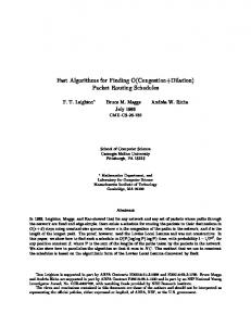
Fig. 1. Eccentricities of vertices in a tree. The two centers in the tree are marked by double circles 5
l l
w(1) = 20 1
2
w(2) = 15
l �� l �� w
w(3) = 12 3
4
(4) = 11
6
7
(5) = 17
(6) = 12 (7) = 17
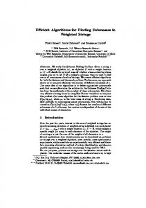
Fig. 2. Weights of vertices in a tree. The unique median in the tree is marked by a double circle.
� median(G) = fi 2 V j w(i) � w(j ) for all j 2 V g denotes the set of medians of G, the set of vertices in V with minimum weight.
Figure 1 shows a tree along with the eccentricity of each vertex. Vertices 3 and 4 have the minimum eccentricity, and are therefore centers of the tree. Figure 2 shows the same tree along with the weight of each vertex. Vertex 4 has the minimum weight, and is therefore the unique median. For the remainder of the paper we restrict our attention to trees. We demonstrate that for this class of graphs, simple and elegant self-stabilizing algorithms for locating centers and medians exist. Our algorithms have been used as the basis of other self-stabilizing algorithms on trees [12, 33]. We hope that our algorithms can be extended to solve the corresponding problems for arbitrary graphs. Let T = (V; E ) be a tree with vertex set V and edge set E . Without loss of generality we assume that V = f1; 2; : : :; ng. The following proposition states well-known properties of centers and medians of trees [3, 4, 17]. Proposition 3.1. A tree has a single center (median) or two adjacent centers (medians).
SELF-STABILIZING ALGORITHMS FOR CENTERS AND MEDIANS
5
3.2. The Model of Computation. Before presenting our self-stabilizing algo-
rithms, we brie y describe the underlying model of computation. We assume that each vertex in T is a process. Each process i maintains a single local variable whose value can be read by the neighboring processes, but can be written into only by i. The program executed by each process is expressed in the language of guarded commands. We assume that each process repeatedly evaluates its guards and checks if any guard is true. If so, the process executes the corresponding action in a single atomic step. Such an atomic step by a process is called a move. A guard that evaluates to true in a certain global state is said to be enabled in that global state. In this model of computation, the execution of our algorithms can be viewed as a sequence of moves, in which moves by di�erent processes are interleaved. In particular, an execution sequence of an algorithm A running on a distributed system S is a sequence: q0 ; m1; q1; m2; q2; : : : such that (i) qi , for each i � 0, is a global state of the system S , (ii) mi , for each i � 1, is a move by some process executing algorithm A, (iii) move mi is a move whose guard is enabled in state qi?1 ; move mi takes the system from state qi?1 into state qi , (iv) the sequence is either in nite or is nite and, if nite, ends in a global state in which no guard is enabled. Since our algorithms are self-stabilizing, no initialization of the variables is assumed. Furthermore, the underlying network topology is permitted to change under the condition that the topology remain connected and acyclic.
3.3. The Algorithms. To facilitate the description of the algorithms, we intro-
duce two functions. Let h : V ! N be a function from vertex set V to the set of natural numbers N . Similarly, let s : V ! N ?f0g be a function from V to the set of positive natural numbers. We will refer to h(i) and s(i) as the h-value and the s-value, respectively, of vertex i. In addition, we will use the following notation: N (i) = fj j (i; j ) 2 E g denotes the set of neighbors of vertex i. Nh (i) = fh(j ) j (i; j ) 2 E g denotes the multi-set of h-values of the neighbors of i. Nh? (i) = Nh (i) ? fmax(Nh(i))g denotes all of Nh (i) with one maximum hvalue removed. For example, if Nh (i) = f2; 3; 3g, then Nh? (i) = f2; 3g.
lh lh lh ls ls ls
SELF-STABILIZING ALGORITHMS FOR CENTERS AND MEDIANS 5
�� l l �� l l �� ��
h(1) = 0 h(2) = 1 1
2
h(3) = 2 h(4) = 2 3
4
6
7
6
(5) = 0
(6) = 1 (7) = 0
Fig. 3. h-values of vertices satisfying the height condition in a tree. 5
l l
s(1) = 1 s(2) = 2 1
2
l �� l ��
s(3) = 3 s(4) = 4 3
4
6
7
(5) = 1
(6) = 3 (7) = 1
Fig. 4. s-values of vertices satisfying the size condition in a tree
Ns(i) = fs(j ) j (i; j ) 2 E g denotes the multi-set of s-values of the neighbors of i. Ns? (i) = Ns (i)?fmax(Ns(i))g denotes all of Ns (i) with one maximum s-value
removed. To motivate our algorithms, we rst make a few observations. The following condition on the h-value of vertex i is called the height condition:
h(i) =
(
0 if i is a leaf ? 1 + max(Nh (i)) otherwise
Here we use the notation max(Nh?(i)) to stand for the maximum value in the multi-set Nh? (i). The following condition on the s-value of a vertex i is called the size condition: ( if i is a leaf s(i) = 11 + �(N ? (i)) otherwise s Here we use the notation �(Ns? (i)) to represent the sum of all the elements in the multi-set Ns? (i).
SELF-STABILIZING ALGORITHMS FOR CENTERS AND MEDIANS
fhCenter- nding algorithm for vertex i g � (i is a leaf) ^ (h(i) 6= 0) ?! ? (i is not a leaf) ^ (h(i) = 6 1 + max(Nh (i))) ?!
h(i) := 0 h(i) := 1 + max(Nh? (i))]
fhMedian- nding algorithm for vertex i g � (i is a leaf) ^ (s(i) 6= 1) (i is not a leaf) ^ (s(i) = 6 1 + �(Ns?(i)))
s(i) := 1 s(i) := 1 + �(Ns? (i))]
?! ?!
7
Fig. 5. The center- nding and the median- nding algorithms
We will show that if the h-values (s-values) of all the vertices in T satisfy the height (size) condition, then the centers (medians) of T are the only vertices whose hvalues (s-values) are greater than or equal to the h-values (s-values) of all neighboring vertices. Figure 3 shows a tree with the h-values of all its vertices satisfying the height condition. The two centers, 3 and 4, are the only vertices whose h-values are greater than or equal to the h-values of all neighbors. Figure 4 shows a tree with the s-values of all its vertices satisfying the size condition. The median, 4, is the only vertex whose s-value is greater than or equal to the s-values of all neighbors. Our center- nding and the median- nding algorithms are shown in Figure 5. It is easy to observe that each of the two statements in the center- nding (median- nding) algorithm is an attempt to ensure that the height (size) condition is satis ed by vertex i.
4. Partial Correctness. The stable states of the center- nding algorithm are
de ned as those that satisfy the height condition. Similarly, the stable states of the median- nding algorithm are those that satisfy the size condition. We prove the partial correctness of the center- nding and median- nding algorithms by showing that the stable states of these algorithms indeed constitute a solution to the center- nding and median- nding problem, respectively. To prove the partial correctness of the proposed algorithms, we introduce the notion of an ordering function. A function f : V ! N , that associates natural numbers to all vertices in T , is an ordering function if for all i 2 V , there exists at most one neighbor j of i such that f (i) � f (j ). We shall refer to f (i) as the f -value of vertex i. The following is easily veri ed (see Figures 3 and 4 for examples). Proposition 4.1. If the h-values (s-values) of all the vertices in T satisfy the height condition (size condition), then h (s) is an ordering function.
SELF-STABILIZING ALGORITHMS FOR CENTERS AND MEDIANS
8
Given an ordering function f : V ! N , de ne a directed graph (digraph) G(f ) = (N (f ); A(f )) whose node1 set is N (f ) = V and whose arc set A(f ) is de ned as:
A(f ) = f(i; j ) j j 2 N (i) and (f (j ); j ) is lexicographically the largestg: Thus, from each node i 2 N (f ) there is an outgoing arc to a neighbor with largest f -value. If there are several neighbors with largest f -value, then the tie is broken by choosing a neighbor with the largest f -value and the largest label. The following lemma states an important property of the digraph G(f ). Lemma 4.2. The underlying undirected graph of the digraph G(f ) is connected. G(f ) contains exactly one cycle and this cycle is of length two. Proof. Since T is connected, by de nition of the arc set A(f ), for all i 2 N (f ), there exists exactly one neighbor of i, say j , such that (i; j ) 2 A(f ). By de nition of an ordering function, for any other neighbor of i, say k, k 6= j , we have f (k) < f (i). Since f (k) < f (i), from the de nition of an ordering function, we conclude that for all neighbors k0 of k, where k0 6= i, f (k0) < f (k). Therefore (k; i) 2 A(f ). This implies that for every edge in T there is at least one corresponding arc in G(f ) and hence G(f ) is connected. Furthermore, every node in G(f ) has exactly one outgoing arc implying that G(f ) has jN (f )j arcs. Since G(f ) is a connected graph with jN (f )j arcs, it contains exactly one cycle. Suppose that (i1; i2; : : :; il) for l � 3 is a cycle in G(f ). We know that if (i; j ) is an arc in A(f ), then (i; j ) is an edge in E . This implies that (i1; i2; : : :; il) is a cycle in T also. But, T is acyclic. Hence, the single cycle that G(f ) contains has to be a 2-cycle (a cycle of length two). Let i and j be the two nodes in G(f ) that belong to its unique cycle. Without loss of generality assume that f (i) � f (j ). On deleting the arcs (i; j ) and (j; i) from G(f ) we obtain two connected components, each of which is a directed tree, with arcs directed towards i and j , respectively. Denote the directed tree containing node i by Ti (f ) = (Ni(f ); Ai(f )) and the directed tree containing node j by Tj (f ) = (Nj (f ); Aj (f )). Designate i as the root of Ti(f ) and j as the root of Tj (f ). Since Ti (f ) and Tj (f ) are now rooted trees, we can use the standard notion of a parent-child relationship between pairs of adjacent nodes in these trees. The following property of the trees Ti (f ) and Tj (f ) is easy to verify. 1 We employ the convention of using \vertex" and \edge" for undirected graphs and \node" and \arc" for directed graphs.
SELF-STABILIZING ALGORITHMS FOR CENTERS AND MEDIANS
9
Proposition 4.3. Each arc in Ti (f ) and in Tj (f ) is directed from a node to its
parent and if k is a non-leaf node in Ti(f ) or in Tj (f ), then f (k) > f (`) for each child ` of k. We now use Proposition 4.1, Lemma 4.2, and Proposition 4.3 to prove the following theorem that provides a way of identifying the centers in T using the h-values associated with the vertices. Theorem 4.4. Let the h-values of all vertices in T satisfy the height condition. Then
center(T ) = fk j h(k) � h(`) for all ` 2 N (k)g: Proof. Since the h-values satisfy the height condition, by Proposition 4.1, h is an ordering function. Hence by Lemma 4.2, G(h) = (N (h); A(h)) is a connected digraph, with a unique cycle that is of length two. Let i and j be the two nodes in the unique cycle in G(h) such that h(i) � h(j ). Consider the rooted, directed trees Ti(h) = (Ni(h); Ai(h)) and Tj (h) = (Nj (h); Aj (h)). It is easy to see that for all k 2 Ni(h) (Nj (h)), h(k) is the height of the subtree of Ti (h) (Tj (h)) rooted at k. The rest of the proof is organized into the following two subcases that are based on the relationship between h(i) and h(j ). Case 1: h(i) > h(j ). In this case, it follows from Proposition 4.3 that i is the only vertex in T whose h-value is greater than or equal to the h-values of all of its neighbors. We will now show that center(T ) = fig. Since h is an ordering function and (i; j ) 2 A(h) we know that j has a largest h-value among all the neighbors of i. Let ` be a child of i in Ti(h) with the largest h-value. Then, h(j ) � h(`). Furthermore, we know that h(i) > h(j ) and h(i) = h(`) + 1. This implies that h(`) = h(j ) and hence h(i) = h(j ) + 1. Since the height of Ti(h) is equal to the distance between the root i and the farthest node from i in Ti(h), we have that e(i) = maxfh(i); h(j ) + 1g = h(i). Similarly, e(j ) = max(h(i) + 1; h(j )g = h(i) + 1. Any node in Ni (h) ? fig is at least a distance of h(j ) + 2 = h(i) + 1 from the farthest node in Tj (h) and any node in Nj (h) ? fj g is at least a distance of h(i) + 2 from the farthest node in Ti(h). This implies that i is the vertex in T with the smallest eccentricity. Hence, center(T ) = fig and the claim in the theorem is true for the case when h(i) > h(j ).
SELF-STABILIZING ALGORITHMS FOR CENTERS AND MEDIANS
10
Case 2: h(i) = h(j ). In this case, Proposition 4.3 implies that i and j are the only
two vertices in T whose h-values are greater than or equal to the h-values of all of their neighbors. We will now show that center(T ) = fi; j g. Furthermore, it is easy to see that e(i) = e(j ) = h(i) + 1 = h(j ) + 1. As in Case 1, any node in Ni (h) ?fig is at least a distance of h(j ) + 2 from the farthest node in Tj (h) and any node in Nj (h) ? fj g is at least a distance of h(i) + 2 from the farthest node in Ti(h). Hence, i and j are the two vertices in T with minimum eccentricity. Therefore, center(T ) = fi; j g. The claim in the theorem is true even in the case when h(i) = h(j ).
Theorem 4.4 implies that if all h-values satisfy the height-condition, then each process can determine if it is a center of T , by simply checking if its h-value is greater than or equal to the h-values of all its neighbors. Thus a stable state of the system running our center- nding algorithm constitutes a solution to the center- nding problem. The following theorem is similar to Theorem 4.4 and provides a way of identifying the medians in T using the s-values of the vertices in T . We omit the proof since it is similar to the proof of Theorem 4.4. Theorem 4.5. Let the s-values of all the vertices in T satisfy the size condition. Then
median(T ) = fk j s(k) � s(`) for all ` 2 N (k)g: Theorem 4.5 implies that if all s-values satisfy the size condition, then each process can determine if it is a median of T or not, by simply checking if its s-value is greater than or equal to the s-values of all its neighbors.
5. Convergence. Our algorithms trivially satisfy the closure property. This is
because in a stable state all guards are false and no moves are possible. This implies that once the system reaches a stable state, it remains in a stable state. So we turn our attention to convergence. To establish convergence of an algorithm, we need to show that any execution sequence of the algorithm is nite in length. In this section we show that any execution sequence of the center- nding algorithm is nite in length, thereby showing that the center- nding algorithm satis es the convergence property. A similar proof (omitted,
SELF-STABILIZING ALGORITHMS FOR CENTERS AND MEDIANS
11
see [23]) su�ces to show that any execution sequence of the median- nding algorithm is also nite. We call a move by process i a decreasing move if it decreases the h-value of process i; otherwise we call the move an increasing move. The convergence proof of the center- nding algorithm is organized in two sections. Section 5.1 shows the total number of decreasing moves that all processes can make is at most n2 . Section 5.2 shows that the total number of increasing moves is also nite. The precise upper bound on the number of increasing moves is established in Section 6.
5.1. Decreasing Moves. We start with an arbitrary execution sequence by the
center- nding algorithm. Let M (i; p) denote a move by process i that is the pth move in this execution sequence. Occasionally, when the identity of the process making a move is irrelevant to our discussion, we will simply use M ( ; p) to denote the move. In what follows, we show that the processes in T can make at most n2 decreasing moves during the execution of the center- nding algorithm. Our proof is presented in two sections. In Section 5.1.1 we de ne the notion of the cause of a decreasing move and prove two properties related to the cause of a decreasing move. Section 5.1.2 extends the notion of the cause of a decreasing move to de ne the source of a decreasing move and then shows that distinct decreasing moves by a process have distinct sources. We then show an upper bound on n on the number of distinct sources and this leads to the upper bound of n on the number of decreasing moves each process can make. The upper bound of n2 on the total number of decreasing moves by all processes follows.
5.1.1. The Cause of a Decreasing Move. Let h(i; p) denote the value of
the variable h(i) after move M ( ; p) and before move M ( ; p + 1). Accordingly, we use Nh? (i; p) to denote the multi-set Nh? (i) after move M ( ; p) and before move M ( ; p +1). Consider a decreasing move M (i; p) by process i. Let us suppose that M (i; p) is not the initial ( rst) move by process i. Intuitively, our goal is to identify a unique neighbor of process i, say j , and a unique decreasing move, say M (j; q ), by process j to be the \cause" of move M (i; p). Since M (i; p) is not the initial move by process i, we can identify a p0 < p such that M (i; p0) is the move made by process i just before move M (i; p). Note that M (i; p0) may or may not be a decreasing move. Focusing on the situation just after move M (i; p0), we notice that since process i has just made a move, (1)
h(i; p0) = max (Nh?(i; p0)) + 1:
SELF-STABILIZING ALGORITHMS FOR CENTERS AND MEDIANS
12
Since move M (i; p) is decreasing, we have that (2)
h(i; p ? 1) > max (Nh?(i; p ? 1)) + 1:
Since M (i; p0) and M (i; p) are consecutive moves by process i, the value of the variable h(i) does not change after move M (i; p0) and before move M (i; p). Hence, h(i; p0) = h(i; p ? 1). This fact, along with (1) and (2), implies that (3)
max (Nh? (i; p ? 1)) < max (Nh?(i; p0)):
It is then easy to see that there exists a neighbor j , of i, such that (4)
h(j; p ? 1) � max (Nh?(i; p ? 1))
and j makes at least one decreasing move between moves M (i; p0) and M (i; p). Furthermore, j itself may have made several decreasing moves between M (i; p0) and M (i; p). Let M (j; q) be the last decreasing move by process j such that p0 < q < p. De ne cause(M (i; p)) = M (j; q ). Note that so far cause() has been de ned only for those decreasing moves that are not initial moves. We extend the de nition to include decreasing moves that are initial, by setting cause(M (i; p)) = M (i; p) if M (i; p) is decreasing and is the initial move by process i. Hence, the cause of a decreasing move by a process is always a decreasing move made by that process or made by a neighbor. We now state and prove two useful properties related to the function cause(). The rst property is that distinct decreasing moves by a process have distinct causes. Lemma 5.1. If M (i; p0) and M (i; p) are distinct decreasing moves by process i then cause(M (i; p0)) 6= cause(M (i; p)). Proof. Without loss of generality assume that p0 < p. Then cause(M (i; p0)) = M ( ; a0) for some a0 � p0 and cause(M (i; p)) = M ( ; a) for some a, p0 < a < p. Thus a0 < a and the lemma follows. The next property that we establish is that the cause relationship is \acyclic." Lemma 5.2. Let M (i; p) be a decreasing move by process i. If M (i; p) is not the initial move by process i, then the move cause(cause(M (i; p))) is not made by process i. Proof. Suppose that M (i; p) is not the initial move of process i. Then there is a neighbor of i, say j , such that cause(M (i; p)) = M (j; q ). If M (j; q ) is the initial move by process j , then cause(M (j; q )) = M (j; q ) and the lemma holds. So we assume that
SELF-STABILIZING ALGORITHMS FOR CENTERS AND MEDIANS
13
M (j; q) is not the initial move by process j . We combine inequalities (2) and (4) to obtain
(5)
h(j; p ? 1) � max (Nh? (i; p ? 1)) < h(i; p ? 1) ? 1:
After the decreasing move M (i; p) we have h(j; p) � max (Nh? (i; p)) = h(i; p) ? 1; implying that h(j; p) < h(i; p). By the same token, if cause(M (j; q )) = M (i; r) for some r < q , then we should have (6)
h(i; q) < h(j; q):
But, we know that h(j; q ) � h(j; p ? 1) because M (j; q ) is the last decreasing move by process j before move M (i; p). In addition, it follows from (5) that h(j; p ? 1) < h(i; p ? 1). We also know that h(i; p ? 1) = h(i; q) because the h-value of process i remains unchanged between moves M (j; q ) and M (i; p). Thus we have,
h(j; q) � h(j; p ? 1) < h(i; p ? 1) = h(i; q); which contradicts inequality (6). Hence, cause(M (j; q )) cannot be a move by process i.
5.1.2. The Source of a Decreasing Move. Based on the de nition of the
cause of a decreasing move, we de ne the notion of the source of a decreasing move. For each decreasing move M (i; p) de ne source(M (i; p)) as follows: 8 > if M (i; p) is decreasing and is > > M (i; p) < move of process i source(M (i; p)) = > source(cause(M (i; p))) iftheM rst ( i; p ) is decreasing, but is > > : not the rst move by process i Intuitively, source(M (i; p)) can be thought of as the initial move that is decreasing and causes M (i; p) through a chain of decreasing moves. Now suppose that
M (i0; p0); M (i1; p1); : : :; M (ia; pa) is a sequence of decreasing moves where (a) M (i0; p0) = M (i; p), (b) M (ia; pa) = source(M (i; p)), and (c) for all b, 0 � b � a ? 1, M (ib+1 ; pb+1) = cause(M (ib ; pb)), and M (ib+1 ; pb+1) 6= M (ib; pb).
SELF-STABILIZING ALGORITHMS FOR CENTERS AND MEDIANS
14
Using Lemma 5.2 and the fact that our algorithm is running on an acyclic network, we conclude that the sequence i0; i1; : : :; ia is a path. Thus, we can associate with each decreasing move M (i; p) a path i0; i1; : : :; ia, called the path to the source of move M (i; p). By inductively applying Lemma 5.1 to paths to the sources of moves M (i; p) and M (i; p0), we easily obtain the following lemma (see [23] for a proof). Lemma 5.3. Let M (i; p0) and M (i; p) be distinct decreasing moves by process i. Then source(M (i; p0)) 6= source(M (i; p)). Since the source of a decreasing move is the rst move by some process, Lemma 5.3 has the following immediate consequence. Corollary 5.4. Each process in T can make at most n decreasing moves. As an immediate consequence we have the following lemma. Lemma 5.5. (Decreasing Moves Lemma) The processes in T can make a total of at most n2 decreasing moves.
5.2. Increasing Moves. In this section we show that the number of increas-
ing moves by the center- nding algorithm is nite. Consider an arbitrary execution sequence of the center- nding algorithm. Since the algorithm can make at most n2 decreasing moves, there exists a nite pre x of the execution sequence that contains all the decreasing moves made by the algorithm. Let the length of the smallest such pre x be t. Hence the execution sequence X = M ( ; t + 1); M ( ; t + 2); M ( ; t + 3); : : : contains only increasing moves. Our goal is to show that X is a nite sequence. Lemma 5.6. (Increasing Moves Lemma) X is a nite sequence. Proof. (by contradiction) To obtain a contradiction, suppose that X is in nite. Clearly, there exists at least one process, say j0, such that in nitely many moves in X are made by j0. Recall that a leaf-process can make at most one move (and that move is decreasing) and hence j0 is not a leaf-process and has at least two neighbors. Clearly, j0 has at least one non-leaf neighbor, say j1, that makes in nitely many moves in X . We will now show that j0 has at least two neighbors that make in nitely many moves in X . Again we show this by contradiction. Suppose that j1 is the only neighbor of j0 that makes in nitely many moves in X . Then, there exists t0 > t such that no neighbor of j0, except j1 , makes moves in the execution sequence
X 0 = M ( ; t0); M ( ; t0 + 1); M ( ; t0 + 2); : : :
SELF-STABILIZING ALGORITHMS FOR CENTERS AND MEDIANS
15
Note that j0 and j1 make in nitely many moves in X 0. Clearly, after nitely many moves in X 0, h(j1) will be strictly greater than the h-value of any other neighbor of j0. This means that after nitely many moves in X 0, Nh? (j0) will no longer contain h(j1) and will therefore subsequently remain unchanged. But if Nh? (j0) remains unchanged, j0 has no reason to make any more moves. The implication is that j0 makes only nitely many moves in X 0 and as a result j0 makes nitely many moves in X . This contradicts our original supposition that j0 makes in nitely many moves in X . Thus j0 has at least two non-leaf neighbors that make in nitely many moves in X . The same is true of j1 and hence we claim that j1 has a non-leaf neighbor j2 , distinct from j0, that makes in nitely many moves in X . This argument can be carried on further to claim the existence of an in nite sequence of distinct non-leaf processes that make in nitely many moves in X . But this is a contradiction because T has a nite number of processes. Hence, our original assumption that X is an in nite execution sequence is false. The Increasing Moves Lemma along with the Decreasing Moves Lemma (Lemma 5.5) leads to the following theorem. Theorem 5.7. Any execution sequence of the center- nding algorithm is nite. This establishes the total correctness of the center- nding algorithm.
6. Time Complexity. In this section we establish upper bounds on the time
complexity of the center- nding and median- nding algorithms. In Section 6.1 we show that the center- nding algorithm makes O(n3 + n2 � ch ) moves in the worst case, where ch is the maximum initial h-value of any process. A similar proof shows that the median- nding algorithm makes O(n3 � cs ) moves in the worst case, where cs is the maximum initial s-value of any process. This proof is omitted (see [23] for the proof). By worst case, we mean a case in which an adversary is allowed not only to maliciously select an initial global state, but is also allowed to choose an execution sequence out of many possible execution sequences. In [12] we show that, when measured in rounds, the time complexity of our center- nding algorithms is �(r), where r is the radius of the tree (eccentricity of the centers). A similar proof su�ces to show that when measured in rounds the time complexity of our median- nding algorithm is �(d), where d is the maximum distance from a median to a leaf.
SELF-STABILIZING ALGORITHMS FOR CENTERS AND MEDIANS
16
6.1. Complexity of the Center-Finding Algorithm. To be speci c, de ne
the global state of the distributed system running the center- nding algorithm to be the n-dimensional vector of natural numbers �
�
h(1); h(2); : : :; h(n) :
Let q be an arbitrary state of the system. We denote the h-value of process i in state q by h(i; q). Accordingly, we use Nh?(i; q) to denote the multi-set Nh?(i) in state q. Given two n-dimensional vectors of natural numbers, q0 and q, we write q0 ! q if there is a move of the center- nding algorithm by some process in T that takes the system from state q0 to state q. As is usual, we use !� to denote the re exive, transitive closure of !. We use q0 !p q to denote that there exists a sequence of p moves of the center- nding algorithm that takes the system from state q0 to state q. Consider two n-dimensional vectors of natural numbers q0 = (h1 ; h2; : : :; hn ) and q00 = (h01; h02; : : :; h0n). We say that q00 dominates q0 (or q0 is dominated by q00) if hi � h0i for all i, 1 � i � n. The next three lemmas are used in Theorem 6.5 to establish an upper bound on the number of moves made by the center- nding algorithm in the worst case. The following lemma can be easily shown by induction on the number of moves required to take the system from state q0 to state q (see [23] for the proof). Lemma 6.1. Suppose that q0 and q00 are states of the center- nding algorithm � q. Then there exists such that q0 is dominated by q00 . Let q be a state such that q0 ! � q0, that dominates q. a state q0, with q00 ! In any state q of the system denote the maximum h-value of any process in T , by hm (q). Let hM (q0) be the maximum h-value of any process in any state that is reachable from q0 . In other words,
hM (q0) = maxfhm (q)) j q0!� qg
We know that hM (q0) exists because we have shown that the center- nding algorithm converges to a state in which all guards are false in a nite number of moves. This implies that every execution sequence starting at q0 is nite in length and hence the number of states reachable from q0 is also nite. Thus hM (q0) is the maximum h-value that any process can achieve when the center- nding algorithm is executed starting in state q0 . The following corollary immediately follows from the above lemma. Corollary 6.2. Let q0 and q00 be states of the center- nding algorithm such that q0 is dominated by q00. Then hM (q0 ) � hM (q00).
SELF-STABILIZING ALGORITHMS FOR CENTERS AND MEDIANS
17
The following lemma uses Corollary 6.2 to establish an upper bound on the maximum h-value reachable from a state q0 = (ch ; ch; : : :; ch), in terms of the maximum h-value reachable from the state q00 = (0; 0; : : :; 0). Since the proof of this lemma is similar to the proof of Lemma 6.1, it is omitted. Lemma 6.3. Suppose that q0 = (ch ; ch; : : :; ch) for some ch 2 N and q00 = (0; 0; : : :; 0). Then hM (q0) � hM (q00 ) + ch . The following lemma establishes a relationship between hm (q0) and hM (q0). Lemma 6.4. Let q0 be a state of T . Then, hM (q0) � hm (q0) + bn=2c. Proof. Let q00 = (hm (q0); hm (q0); : : :; hm(q0 )). Since q0 is dominated by q00, by Corollary 6.2, hM (q0) � hM (q00). Now let q000 = (0; 0; : : :; 0). By Lemma 6.3, hM (q00) � hM (q000 )+hm(q0). This leads to the inequality hM (q0) � hM (q000)+hm (q0). It is easy to see that an upper bound on hM (q000) is bn=2c. Theorem 6.5. The center- nding algorithm can make at most O(n3 + n2 � hm (q0 )) moves starting from state q0. � q. Let H (q) be the sum of the h-values of Proof. Let q be a state such that q0! all the processes in state q. Thus H (q) = �i2V h(i; q). Clearly, 0 � H (q) � nhM (q0 ), for all q, with q0 !� q. If the center- nding algorithm makes no decreasing moves, then an upper bound on the total number of increasing moves is nhM (q0). But the algorithm may make up to n2 decreasing moves and each decreasing move may reduce the value of H () by at most hM (q0). Hence, the total amount of reduction that the decreasing moves can cause is at most n2 hM (q0). Thus an upper bound on the total number of increasing moves is nhM (q0 ) + n2 hM (q0 ). Using Lemma 6.4 this bound can be translated into (hm (q0) + bn=2c)(n + n2 ). Thus, including decreasing moves, the center- nding algorithm can make at most O(n3 + n2 � hm (q0)) moves.
7. Extensions. It is easy to extend the center- nding and median- nding al-
gorithms to trees with arbitrary, positive edge-costs. In particular, suppose that c(i; j ) 2