Author manuscript, published in "POLINSAR 2009, Frascati : Italie (2009)"
Segmentation and Classification of Polarimetric SAR Data based on the KummerU Distribution Olivier Harant∗† , Lionel Bombrun∗ , Michel Gay∗ , Renaud Fallourd‡ , Emmanuel Trouv´e‡ , Florence Tupin§ ∗ Grenoble
hal-00449236, version 1 - 21 Jan 2010
Image Parole Signal et Automatique (GIPSA-lab), CNRS INPG - 961, Rue de la Houille Blanche - BP 46 - 38402 Saint-Martin-d’H`eres, France Email:
[email protected] † IETR Laboratory, SAPHIR Team, University of Rennes 1, Bat. 11D, 263 avenue du G´en´eral Leclerc 35042 Rennes, France ‡ LISTIC - Polytech’Savoie, 74944 Annecy le Vieux, France § Institut TELECOM, TELECOM ParisTech, CNRS LTCI, 46 rue Barrault, 75634 Paris, France
Abstract—Thinner spatial features can be observed from the high resolution of newly available spaceborne and airborne SAR images. Heterogeneous clutter models should be used to model the covariance matrix because each resolution cell contains only a small number of scatterers. In this paper, we focus on the use of a Fisher probability density function (pdf) to model the SAR clutter. First, the benefit of using such a pdf is exposed. Covariance matrix statistics are then analysed in details. For a Fisher distributed texture, the covariance matrix follows a KummerU pdf. Asymptotic cases of this pdf are presented. Finally, the KummerU pdf is implemented in both hierarchical segmentation and classification algorithms. Segmentation and classification results are shown on both synthetic and real data.
I. I NTRODUCTION Synthetic Aperture Radar (SAR) data are the result of a coherent imaging system that produces the speckle noise phenomenon. For multi-look multichannel Polarimetric SAR (PolSAR) data, the covariance matrix is used to characterize the scatterers. For fully developed speckle, the covariance L 1X matrix, Zh = ~xhk ~x†hk follows the complex Wishart L k=1 distribution [1]. It is assumed that land cover backscatter characteristics are homogeneous (denoted by subscript h) over the area. However, thinner spatial features can be observed from the high resolution of newly available spaceborne and airborne SAR images. In this case, heterogeneous clutter models should be used because each resolution cell contains only a small number of scatterers. First, authors propose to model the PolSAR texture parameter by a Fisher pdf. As the Fisher pdf has an hybrid behavior between a Gamma pdf and an Inverse Gamma pdf, it has been successfully applied in high resolution SAR images to model the SAR clutter [2]. For such a clutter, the covariance matrix follows a KummerU pdf [3]. A details analysis of the asymptotic cases of the KummerU pdf is carried out. Next, this pdf is implemented in a hierarchical segmentation algorithm. Then, authors propose to adapt the Wishart classifier to the KummerU distribution. Segmentation and classification results are shown on both synthetic and real data.
In this paper, authors work with L-look PolSAR data. Those images are characterized in terms of covariance matrix. Mathematical relations exposed in this paper can be easily adapted for 1-look data (described by the target vector ~x). II. T EXTURE MODELING A. The scalar product model For textured areas, the “product model” has been proposed [4]. The observed covariance matrix Z can be written as the product of a texture parameter µ with the covariance matrix for homogeneous surface Zh , Z = µ Zh . Generally the texture is polarimetric dependent and µ is represented by a matrix. Here, µ is assumed to be a positive scalar parameter. The texture term is generally modeled by a Gamma pdf. The observed signal then follows a K distribution. Recent works have proposed to model the texture parameter by a Fisher pdf defined by three parameters L, M and m as : µ F [m, L, M] =
Lµ Mm
¶L−1
Γ(L + M) L µ ¶L+M Γ(L)Γ(M) Mm Lµ 1+ Mm
(1)
Under the scalar product model assumption, it follows that the covariance matrix distribution can be expressed by means of the confluent hypergeometric function of the second kind (KummerU), and this distribution has been named the KummerU pdf [3] :
LLp |Z|L−p Γ(L + M) K(L, p)|Σh |L Γ(L) + Γ(M) µ ¶Lp L Γ(Lp + M) U (a, b, z) Mm
pZ (Z|Σh , L, M, m) =
p(p−1)
(2)
where K(L, p) = π 2 Γ(L) . . . Γ(L − p + 1) is a normalization factor. L and p are respectively the number of look and data dimension (p = 3 for the reciprocal case), Pthe L Z = L1 k=1 Zk is the mean coherency matrix and U (a, b, z)
is the confluent hypergeometric function of the second kind −1 Z)L h (named KummerU) with z = LTr(ΣMm , a = Lp + M, b = 1 + Lp − L. | · | and Tr(·) are respectively the determinant and trace operator.
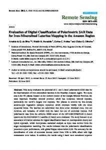
With high resolution images of man-made objects, the Fisher distribution has been successfully introduced to model the SAR clutter [2]. To show the benefit of using Fisher pdf to model the texture parameter, an urban area (50 × 50 pixels) has been extracted from the 8-look L-band PolSAR image over the Oberpfaffenhofen test-site. Then, the empirical texture distribution is modeled by Gamma and Fisher pdf (Figure 1). Fisher pdf (red and blue lines) provide a better modeling of this clutter than Gamma pdf (green line). Moreover, Fisher parameters estimated by the log-moment method fit better the empirical distribution than the moment based method. In the following, Fisher parameters will be estimated by the logmoment method.
¡ ¢ L−Lp LLp |Z|L−p h L tr Σh −1 Z i 2 pZ (Z|Σh , L, M, m) = K(L, p)|Σh |L L µ q ¶ L ¡ −1 ¢ 2L × BesselKL−Lp 2 LL tr Σh Z (5) Γ(L)
0.02 0.018 covariance matrix pdf
hal-00449236, version 1 - 21 Jan 2010
B. Benefit of Fisher pdf
1) For large M: the Fisher pdf has the same behavior as a Gamma pdf. Abramowitz and Stegun have shown the following relation [5, Eq. 13.3.3] which links an asymptotic case of the KummerU function with the K-Bessel function of the second kind (noted BesselK): √ b 1 lim {Γ(1 + a − b)U (a, b, z/a)} = 2 z 2 − 2 BesselKb−1 (2 z) a→∞ (4) If we replace a,¡ b and z¢ respectively by Lp+M, 1+Lp−L −1 Z , one can easily proved that for large and Lp+M Mm LL tr Σh M, the KummerU pdf tends toward the well-known K pdf [6] [7] defined by :
1.2
empirical Fisher distribution (moments) Fisher distribution (log moments) Gamma distribution
1
0.8
0.016 0.014 0.012 0.01
0.6
0.008
0
20
0.4
Fig. 2.
0.2
0 0
Fig. 1.
0.5
1
1.5
2
2.5
3
3.5
Convergence of the KummerU pdf toward the K pdf
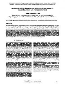
Figure 2 shows the convergence of the KummerU pdf (Fisher distributed clutter) toward the K pdf (Gamma distributed clutter) as a function of the M Fisher parameter.
4
Texture Modeling of an urban clutter by Gamma and Fisher pdf
C. Particular cases of the KummerU pdf Fisher pdf have been introduced by means of second kind statistics and Mellin transform. It can be shown that the Fisher pdf (F [m, L, M]) is equal to the Mellin convolution of a Gamma pdf (G [m, L]) by an Inverse Gamma pdf (GI [1, M]). F [m, L, M] = G [m, L] ˆ? GI [1, M]
40 60 M Fisher parameter
KummerU pdf K pdf 80 100
(3)
Consequently, Fisher pdf have an hybrid behavior between those two pdf. In this part, authors propose to study the asymptotic cases of the KummerU pdf.
2) For large L: the Fisher pdf has the same behavior as a Gamma Inverse pdf. It can be shown that for a Gamma Inverse distributed texture, the covariance matrix follows a pdf defined by : pZ (Z|Σh , M) = ×
LLp |Z|L−p
MM p(p−1) π 2 Γ(L) · · · Γ(L − p + 1)|Σh |L Γ(M) ³ ´−(M+Lp) ¡ ¢ Γ(Lp + M) L tr Σh −1 Z + M (6)
Figure 2 shows the convergence of the KummerU pdf (Fisher distributed clutter) toward the covariance matrix pdf for a Gamma Inverse distributed clutter as a function of the L Fisher parameter. As the Fisher pdf is a generalization of the Gamma pdf, the KummerU pdf can be viewed as a generalization of the
Covariance matrix pdf
12 x 10
−3
11 10 9 8 7 0
20
texture 2 L=5 M=30 m=1
texture 3 L=10 M=10 m=1
texture 4 L=10 M=30 m=1 (a)
KummerU pdf For a Gamma Inverse clutter 40 60 80 100 L Fisher parameter
(b)
Fig. 4. (a) Image containing the 4 segments (ground truth) and Fisher parameters used in the simulation (b) 4-areas synthetic texture image (200 × 200)
Fig. 3. Convergence of the KummerU pdf toward the covariance matrix pdf for a Gamma Inverse clutter
hal-00449236, version 1 - 21 Jan 2010
texture 1 L=5 M=10 m=1
K pdf. The KummerU pdf is therefore well adapted to fit a large range of clutter, especially for high resolution PolSAR data. In the following, authors propose to implement this pdf in both statistical segmentation and classification algorithms. III. H IERARCHICAL SEGMENTATION A. Principle Hierarchical segmentation consists in dividing iteratively an image into several segments. The image is initially divided into a large number of segments (typically, one pixel is one segment). At each iteration, a similarity measure is computed for each 4-connex segment pair. Then, the two segments which minimizes this similarity is merged to create a new segments. Those two steps are repeated iteratively until the desired number of segments in the final partition is reached. The similarity measure selected here is based on the log-likelihood function. For two adjacent segments Si and Sj , the stepwise criterion SCi,j is equal to the decrease of log-likelihood induced by the merging. This criterion is defined by [8]:
2) For high resolution PolSAR images : the texture parameter can be modeled by a Fisher pdf. Under the scalar product model, the covariance matrix follows a KummerU pdf (Eq. 2). The log-likelihood function for segment S is defined by : n o n o ˆ − n ln Γ(L) ˆ MLL(S) ≈ − nL ln |Ch | + n ln Γ(Lˆ + M) Ã ! n o n o ˆ L ˆ + nLp ln ˆ − n ln Γ(M) + n ln Γ(Lp + M) ˆm M ˆ ( Ã ¡ −1 ¢ !) X L tr Ch Zk Lˆ ˆ 1 + Lp − L; ˆ + ln U Lp + M; ˆm M ˆ Zk ∈S (9) ˆ M ˆ and m where L, ˆ are respectively the estimated of the Fisher parameters L, M and m by the log-cumulants method [2] [9]. Ch is the best likelihood estimate of Σh for segment S. The first term in Eq. 9 (nL ln |Ch |) corresponds to the log-likelihood function for a Wishart pdf. All other terms in Eq. 9 are introduced by the use of a Fisher pdf to model the texture of PolSAR images. B. Segmentation results
SCi,j = MLL(Si ) + MLL(Sj ) − MLL(Si ∪ Sj )
(7)
where MLL(·) is the maximum log-likelihood function. 1) For a fully developed speckle : the covariance matrix is modeled by a Wishart pdf, the stepwise criterion is therefore equal to [8] :
SCi,j = L(ni + nj ) ln |CSi ∪Sj | − Lni ln |CSi | − Lnj ln |CSj | where CSi is the mean covariance matrix computed over the ni pixels of segment Si . It is the best likelihood estimated of Σ for segment Si .
In this part, authors propose to evaluate the segmentation performance of both Wishart and KummerU criteria. Here, a synthetic PolSAR data set is created. This data set is composed of 4 quadrants. In each quadrants (100 × 100 pixels), Fisher realizations are generated to model the clutter. Then, the same Wishart pdf is used to model the speckle over the whole image. The PolSAR data set is obtained by multiplying the texture image by speckle one. Figure 4 shows the PolSAR data set : (8) To compute statistics on texture, authors have decided to execute the hierarchical segmentation algorithm with an initial partition where each segment is a bloc of 10 × 10 pixels. Figure 5 shows segmentation results for both Wishart and KummerU criteria.
KummerU
Wishart
20
20
40
40
60
60
80
80
100
100
120
120
140
140
160
160
180
By following the same procedure as [10], one can derive the KummerU distance for segment S to the ath class :
180
200
200 20
40
60
80
100
120
140
160
180
200
20
40
60
80
100
120
140
160
180
Fig. 5. Hierarchical segmentation results with both modeling KummerU (left) and Wishart (right) computed on image 4
200
dKummerU (Z, {Σha , La , Ma , ma }) = nL ln |Σha | −n ln {Γ(La + Ma )} + n ln {Γ(La )} ¶ µ La − n ln {Γ(Lp + Ma )} + n ln {Γ(Ma )} − nLp ln Ma ma ( Ã ¡ ¢ !) P L tr Σha −1 Zk La − ln U Lp + Ma ; 1 + Lp − La ; Ma ma Zk ∈S where La , Ma and ma are the Fisher parameters of the ath class. Then, segment S is affected to the a ˆth class if the KummerU distance is minimized : a ˆ = Argmin dKummerU (Z, {Σha , La , Ma , ma })
(11)
a
hal-00449236, version 1 - 21 Jan 2010
B. Classification results (a) Initial segmentation
(b) Wishart
(c) KummerU
Fig. 6. Hierarchical segmentation results with both modeling KummerU (center) and Wishart (right) computed on fully developed speckle dataset composed by four Wishart pdf divided into 10 × 10 pixels segments.
Segmentation using Wishart criterion drives to a quite wrong segmentation. Whereas segmentation using KummerU criterion give suitable results: excepting few segments which are wrong, each quadrant is well segmented. Indeed, for this data set, the Wishart criterion is not adapted because the speckle is not fully developed. Consequently, segmentation results based on the Wishart criterion are not accurate. To evaluate the performance of the KummerU criterion, authors have generated another data set. This data set represents a fully developed speckle, no texture is used in the simulation. It is composed only by four Wishart pdf, one in each quadrant. Figure 6 illustrates that both Wishart and KummerU criteria succeed in segmenting this data set.
In this part, authors propose to evaluate classification performance of Wishart and KummerU criteria. We have generated a synthetic data set composed by 4 classes. For each class, a Fisher pdf has been used to model the clutter. Fisher parameters used in the simulation can be found in Fig. 7(a). Then, the speckle has been generated by using the same Wishart over the 4 classes. The PolSAR data set is obtained by multiplying the texture image (Fig. 7(b)) by the speckle one. texture 1 L=2 M=2 m= 12
texture 2 L=2.1 M=3 m= 23
texture 3 L=2.2 M=4 m= 34
texture 4 L=2.3 M=5 m= 45 (a)
(b)
Fig. 7. (a) Image composed by 4 classes and Fisher parameters used in the simulation (b) 4-areas synthetic texture image (200 × 200)
IV. C LASSIFICATION A. Principle In this part, authors propose to adapt the Wishart classifier to the KummerU pdf. For a fully developed speckle, the covariance matrix follows a Wishart pdf. The Wishart distance used in the classification algorithm is obtained by computing the log-likelihood function [10] : ³ ´ dWishart (Z, Σha ) = ln |Σha | + tr Σ−1 Z ha
(10)
where Σha = E {Z|Z ∈ ωa }, ωa is the set of pixels belonging to the ath class.
In this simulation, the four Fisher pdf have the same mean M value m1 = m = 1. Classifying such a data set is M−1 hard task. Table I shows Wishart and KummerU criteria for a population (50 × 50 pixels) belonging to class 1. Both Wishart and KummerU criteria succeed in classifying this population to class 1. TABLE I W ISHART AND K UMMERU CRITERIA FOR A POPULATION BELONGING TO CLASS 1 Criterion Wishart KummerU
class 1 1.253 9.309
Distances class 2 1.256 9.329
(×105 ) class 3 1.258 9.383
class 4 1.259 9.438
well adapted to fit a large range of clutter, especially for high resolution PolSAR data. Under the scalar product model assumption, the covariance matrix follows the KummerU pdf [3]. In this paper, authors have presented some asymptotic cases of the KummerU pdf. For example, for large M, we retrieve the K pdf, which supposed a Gamma distributed clutter. Therefore, the KummerU pdf can be viewed as a generalization of many distributions and gives at least as good performance as standard pdf. Then, authors have proposed to implement this distribution in both hierarchical segmentation and classification algorithms. Segmentation and classification results are shown on both synthetic and real data.
(a) KummerU
hal-00449236, version 1 - 21 Jan 2010
8 100
7
200
6
300
5
400
4
500
3
600
2 1
700 100
200
300
400
500
600
700
(b) Fig. 8. (a) Colored composition in the Pauli basis of a PolSAR image over the Oberpfaffenhofen test site (b) Classification results in 8 classes for the KummerU criterion
After having presented some results on synthetic images, we show classification results over the L-band 8-look PolSAR image over the Oberpfaffenhofen test site. Figure 8(a) shows a colored composition in the Pauli basis of the covariance matrix. The classification algorithm process starts with an initial partition. This partition is issued from the hierarchical segmentation algorithm based on the KummerU criterion [3]. Here, we have decided to start with an initial partition composed by 10 000 segments. Next, we compute the KummerU criterion for segment S to each class. Then, segment S is affected to class which minimized the KummerU criterion. Those steps are repeated iteratively until maximum a number of iterations is reached. Figure 8(b) shows the classification map into 8 classes obtained with the KummerU classifier. V. C ONCLUSION In this paper, authors have focused on the use of texture to extract information from PolSAR data. The Fisher pdf has been chosen to model the PolSAR clutter. Like this pdf can model distributions with either heavy head or heavy tail, it is
In perspectives of this work, authors propose to apply the SIRV estimation scheme in the hierarchical segmentation algorithm. In this case, the Fixed Point estimator is used to estimate the normalized coherency matrix Σh . As this estimator is independent on the texture pdf, it will be of great interest to compare the segmentation performance between those two algorithms. R EFERENCES [1] N. Goodman, “Statistical analysis based on a certain multivariate complex Gaussian distribution (an introduction),” in Ann. Math. Statist., vol. 34, 1963, pp. 152–177. [2] C. Tison, J.-M. Nicolas, F. Tupin, and H. Maˆıtre, “A New Statistical Model for Markovian Classification of Urban Areas in High-Resolution SAR Images,” IEEE Transactions on Geoscience and Remote Sensing, vol. 42, no. 10, pp. 2046–2057, October 2004. [3] L. Bombrun and J.-M. Beaulieu, “Fisher Distribution for Texture Modeling of Polarimetric SAR Data,” IEEE Geoscience and Remote Sensing Letters, vol. 5, no. 3, Juillet 2008. [4] I. Joughin, D. Winebrenner, and D. Percival, “Polarimetric Density Functions for Multilook Polarimetric Signatures,” IEEE Transactions on Geoscience and Remote Sensing, vol. 32, no. 3, pp. 562–574, 1994. [5] M. Abramowitz and I. Stegun, Handbook of Mathematical Functions With Formulas, Graphs, and Mathematical Tables, 1964. [6] J. Lee, D. Schuler, R. Lang, and K. Ranson, “K-Distribution for MultiLook Processed Polarimetric SAR Imagery,” in Geoscience and Remote Sensing, IGARSS ’94, Seoul, Korea, 1994, pp. 2179–2181. [7] A. Lop`es and F. S´ery, “Optimal Speckle Reduction for the Product Model in Multilook Polarimetric SAR Imagery and the Wishart Distribution,” IEEE Transactions on Geoscience and Remote Sensing, vol. 35, no. 3, pp. 632–647, 1997. [8] J.-M. Beaulieu and R. Touzi, “Segmentation of Textured Polarimetric SAR Scenes by Likelihood Approximation,” IEEE Transactions on Geoscience and Remote Sensing, vol. 42, no. 10, pp. 2063–2072, 0ctober 2004. [9] J.-M. Nicolas, “Application de la transform´ee de Mellin: e´ tude des lois statistiques de l’imagerie coh´erente,” in Rapport de recherche, 2006D010, 2006. [10] J. Lee, M. Grunes, T. Ainsworth, L. Du, D. Schuler, and S. Cloude, “Unsupervised Classification Using Polarimetric Decomposition and the Complex Wishart Classifier,” IEEE Transactions on Geoscience and Remote Sensing, vol. 37, no. 5, pp. 2249–2258, 1999.