Three-Dimensional Sound Source Localization for Unmanned Ground

Proceedings of the 5th International Conference of Control, Dynamic Systems, and Robotics (CDSR'18) Niagara Falls, Canada – June 7 – 9, 2018 Paper No. 104 DOI: 10.11159/cdsr18.104

Three-Dimensional Sound Source Localization for Unmanned Ground Vehicles with a Self-Rotational Two-Microphone Array Deepak Gala, Nathan Lindsay, Liang Sun New Mexico State University 1780 E University Ave, Las Cruces, New Mexico, USA [email protected]; [email protected]; [email protected] Abstract - This paper presents a novel three-dimensional (3D) sound source localization (SSL) technique based on only Interaural Time Difference (ITD) signals, acquired by a self-rotational two-microphone array on an Unmanned Ground Vehicle. Both the azimuth and elevation angles of a stationary sound source are identified using the phase angle and amplitude of the acquired ITD signal. An SSL algorithm based on an extended Kalman filter (EKF) is developed. The observability analysis reveals the singularity of the state when the sound source is placed above the microphone array. A means of detecting this singularity is then proposed and incorporated into the proposed SSL algorithm. The proposed technique is tested in both a simulated environment and two hardware platforms, i.e., a KEMAR dummy binaural head and a robotic platform. All results show the fast and accurate convergence of estimates. Keywords: Sound Source Localization, Spatial Hearing, Extended Kalman Filter (EKF), Interaural Time Difference

(ITD).

1. Introduction Exploring in an unknown environment is still a challenging task for an unmanned vehicle without the support of the Global Positioning System (GPS). Computer vision is the most popular method used nowadays for mobile robots to “sense” and “perceive” the environment and identify its position in a GPS-denied environment. However, the sensing capability of a visual sensor is largely degraded when the object of interest is out of its field of view or when the lighting condition is poor. In these situations, computer hearing, supported by inexpensive acoustic sensors, can provide valuable situational awareness because the sound is less affected by obstacles nor depends on lighting conditions. Also, computer hearing plays an important role in human-robot interaction and has evolved as an independent scientific research area of its own in the past 15 years. It is significant for humanoid robots to have hearing capability to communicate in the same way as humans. This will make the robots more sociable and more acceptable by the humans. Sound source localization (SSL), as a major branch in computer hearing, has been witnessed in applications ranging from an intelligent video conferencing [1] to advanced military applications [2]. SSL plays a significant role for humanoid robots to become more powerful in autonomous tasks [3]. In the past, research has been conducted for localization of sound sources using interaural time difference (ITD), interaural level difference (ILD), and spectral cues [4]–[12]. Most of these techniques are based on microphone arrays with more than two microphones [9]–[12]. The performance of microphone arrays is largely dictated by the physical size and placement of microphones [11]. The requirement of having a certain and fixed geometry makes it difficult for microphones to be installed on robots [12]. While there are techniques localizing sound sources in a two-dimensional (2D) space [13], [14], three-dimensional (3D) localization techniques have also been developed but with laborious processes [5]–[8]. A majority of the research for SSL is based on the head related transfer function (HRTF) which uses spectral cues [4]–[6]. 3D SSL techniques using ITD cues either demand complicated calculations [8] or showing inconsistent and large estimation errors [7]. To the best of our knowledge, no research has been reported in the literature that directly estimates the location information (e.g., elevation and azimuth angles) of a sound source using the characteristics (i.e., amplitude and phase) of ITD signals acquired by a self-rotational two-microphone array. The major contribution of this paper is a novel 3D localization technique that estimates the location of a stationary sound source in a spherical coordinate frame. The proposed technique works with a binaural device (e.g., a dummy head) as well as a robot with only two microphones rotating around their geometric center, as shown in Fig. 1. The proposed

104-1

technique is developed based on the insight that the rotation of the two-microphone array leads to a sinusoidal ITD signal. The phase shift of the resulting sinusoidal signal can be directly mapped to the azimuth angle of the sound source, and the amplitude of the ITD signal can be represented as a function of the elevation angle of the sound source and the distance between the two microphones. An extended Kalman filter (EKF) is developed to handle the sensor noise when estimating the amplitude and phase-shift of the ITD signal, which in turn results in the calculation of the azimuth and elevation angles of the sound source in a 3D environment. The proposed technique is validated using both simulated and experimental data and the results show its effectiveness.

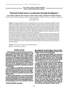
Fig. 1: Robotic platform with two MEMS microphones.

The reminder of this paper is organized as follows. Section 2 presents the preliminaries. In Section 3, a 3D model of the proposed SSL system is presented. The extraction of location information from the ITD signal characteristics is presented in Section 4. In Section 5, the observability analysis and the EKF development are presented. Simulation and experimental results are presented and discussed in Sections 6 and 7, respectively. Section 8 concludes the paper.

2. Preliminaries Consider a two-microphone array separated with a constant distance. Let 𝑦1 (𝑡) and 𝑦2 (𝑡) be the signals received by the two microphones aroused by a single sound source, which are given by 𝑦1 (𝑡) = 𝑠(𝑡) + 𝑛1 (𝑡) and 𝑦2 (𝑡) = 𝛿 ⋅ 𝑠 (𝑡 + 𝑡𝑑 ) + 𝑛2 (𝑡), where 𝑡𝑑 is the time difference of arrival (TDOA), i.e., the ITD, of 𝑦1 (𝑡) and 𝑦2 (𝑡), 𝑠 (𝑡) is the sound signal produced by the sound source, 𝑛1 (𝑡) and 𝑛2 (𝑡) are real and jointly stationary random processes, and 𝛿 is the signal attenuation factor due to different traveling distances of the sound signal to the two microphones. It is commonly assumed that 𝛿 changes slowly and 𝑠(𝑡) is uncorrelated with noises 𝑛1 (𝑡) and 𝑛2 (𝑡) [15]. Then, the ITD (𝑡𝑑 ) of 𝑦1 and 𝑦2 can be calculated using cross correlation [15]. 𝑅𝑦1,𝑦2 (𝜏) = 𝐸[ 𝑦1 (𝑡). 𝑦2 (𝑡 − 𝜏)],

(1)

where 𝐸 [⋅] represents the expectation operation.

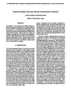
Fig. 2: Calculation of the Interaural Time Delay (ITD) between two signals 𝑦1 (𝑡) and 𝑦2 (𝑡) using cross-correlation.

Fig. 2 shows the calculation process of ITD between 𝑦1 (𝑡) and 𝑦2 (𝑡), where 𝐻1 (𝑓) and 𝐻2 (𝑓) represent scaling functions or pre-filters used to eliminate or reduce the effect of background noise and reverberations [16]–[17]. The

104-2

improved version of the cross-correlation method incorporating 𝐻1 (𝑓) and 𝐻2 (𝑓), i.e., the Generalized Cross-Correlation (GCC) can be found in [15]. The estimate of the ITD between 𝑦1 (𝑡) and 𝑦2 (𝑡) is given by 𝑇̂ ≜ arg max 𝑅𝑦1,𝑦2 (𝜏). 𝜏

(2)

The difference of the traveling distances of the sound signal to the two microphones is then given by 𝑑̂ = 𝑇̂ . 𝑐0 , where 𝑐0 is the sound speed.

3. Three-Dimensional Model for SSL In this paper, the location of the sound source is defined in a spherical coordinate frame, whose origin locates at the centre of the two microphones equipped on a ground robot. The focus of this paper is to identify the azimuth and elevation angles of the sound source with respect to the robot body frame, while the identification of the distance between the sound source and the robot is out of the scope of this paper.

Fig. 3: Top-down view of the system.

. Fig. 4: 3D view of the system.

Fig. 5: Top-down view of the plane containing triangle SOF.

104-3

As shown in Figs. 3 and 4, the acoustic signal generated by the sound source 𝑆 is collected by the left and right microphones, 𝐿 and 𝑅, respectively. Let 𝑂 be the center of the two microphones. The location of the sound source is 𝜋 represented by (𝐷, 𝜃, 𝜑), where 𝐷 is the length of segment 𝑂𝑆, 𝜃𝜖 [0, 2 ] is the elevation angle defined as the angle between 𝑂𝑆 and the horizontal plane, and 𝜓 𝜖 [−𝜋, 𝜋] is the azimuth angle defined as the angle measured clockwise from the robot heading vector, 𝐩, to 𝑂𝑆. Letting unit vector 𝐪 be the orientation (heading) of the microphone array, 𝛽 be the angle between 𝐩 and 𝐪, and ѱ be the angle between 𝐪 and 𝑂𝑆, both following a right-hand rotation rule, we have 𝜑 = 𝜓 + 𝛽.

(3)

In the shaded triangle, ∆𝑆𝑂𝐹, shown in Figs. 4 and 5, define 𝛼 = ∠ 𝑆𝑂𝐹 and we have cos 𝛼 = cos 𝜃 sin 𝜓. Based on the far-field assumption [18], we have 𝑑 ≜ 𝑇̂. 𝑐0 = 2𝑏 cos 𝛼 = 2𝑏 cos 𝜃 sin 𝜓.

(4)

4. Identification of Azimuth and Elevation Angles of a Sound Source To avoid cone of confusion [19] in SSL, the two-microphone array is rotated with a nonzero angular velocity [7]. Without loss of generality, in this paper we assume a clockwise rotation of the microphone array on the horizontal plane while the robot itself does not rotate nor move throughout the entire estimation process, which implies that 𝜑 is constant. The initial heading of the microphone array is configured to coincide with the heading of the robot, i.e., 𝛽(𝑡 = 0) = 0, which implies that 𝜑 = 𝜓(0). As the microphone array rotates clockwise with a constant angular velocity, 𝜔, we have 𝛽(𝑡) = 𝜔𝑡 and due to Eqn. (3) we have 𝜓(𝑡) = 𝜑 − 𝛽(𝑡) = 𝜑 − 𝜔𝑡.

(5)

The resulting time-varying 𝑑(𝑡) due to Eqn. (4) is then given by 𝑑(𝑡) = 2𝑏 cos 𝜃 sin(−𝜔𝑡 + 𝜑).

(6)

Because the microphone array rotates on the horizontal plane, 𝜃 does not change during the rotation for a stationary sound 𝐴 source. The resulting 𝑑 (𝑡) is a sinusoidal signal with the amplitude 𝐴 ≜ 2𝑏 cos 𝜃, which implies that 𝜃 = 𝑐𝑜𝑠−1 . The 2𝑏 phase angle of 𝑑 (𝑡) is the azimuth angle of the sound source. Therefore, the localization of a stationary sound source equates the identification of the characteristics (i.e., the amplitude and phase angle) of the sinusoidal signal, 𝑑 (𝑡).

5. Estimation of ITD Signal Characteristics Using EKF Although a least square approach could be used to estimate the elevation and azimuth angles of a stationary sound source, an EKF model is developed towards implementing a platform that can be extended for a moving source and a mobile robot. 5.1. State-Space Model Defining 𝑥 ≜ [ 𝐴, 𝜑, 𝛽 ]𝑇 as the state vector, the process function is given by 𝑥̇ = 𝑓(𝑥) = [0 0 𝜔]𝑇 , and the output function is given by

104-4

(7)

𝑦 = ℎ(𝑥) = [

𝐴 sin(𝜑 − 𝛽) ]. 𝛽

(8)

Since the rotation of the microphone array is controlled by the robot, it implies that the angle 𝛽 is directly measurable. 5.2. Observability Analysis Theorem 1. The state 𝑥 = [ 𝐴, 𝜑, 𝛽 ]𝑇 associated with Eqns. (7) and (8) is observable if 1) 𝐴 ≠ 0 and 2) 𝜔 ≠ 0. Proof: To calculate the observability matrix [20] of the state-space nonlinear system described by Eqns. (7) and (8), the following Lie derivatives [20] are needed. 𝐿𝑓0 ℎ = ℎ(𝑥) = [ 𝐿1𝑓 ℎ =

𝜕𝐿𝑓0 ℎ 𝜕𝑥

𝐴 sin(𝜑 − 𝛽) ], 𝛽

(9)

−𝐴𝜔 cos(𝜑 − 𝛽) 𝑓=[ ]. 𝜔

(10)

The observability matrix is then given by 𝜕𝐿0 ℎ Ω = [( 𝑓 ) 𝜕𝑥

𝑇

𝑠(𝜑−𝛽) 𝑇 𝑇 𝜕𝐿1𝑓 ℎ 0 ( ) ] = [−𝜔 𝑐 (𝜑−𝛽) 𝜕𝑥 0

𝐴 𝑐(𝜑−𝛽) 0 𝐴 𝜔 𝑠(𝜑−𝛽) 0

−𝐴 𝑐(𝜑−𝛽) 1 ], −𝐴 𝜔 𝑠(𝜑−𝛽) 0

(11)

where 𝑠(𝜑−𝛽) = sin(𝜑 − 𝛽) and 𝑐(𝜑−𝛽) = cos(𝜑 − 𝛽). Consider the matrix consisting of the first three rows of Ω 𝑠(𝜑−𝛽) 0 Ω =[ −𝜔 𝑐(𝜑−𝛽) ′

𝐴 𝑐(𝜑−𝛽) 0 𝐴 𝜔 𝑠(𝜑−𝛽)

−𝐴 𝑐(𝜑−𝛽) 1 ], −𝐴 𝜔 𝑠(𝜑−𝛽)

(12)

′

and the determinant of Ω′ is det(Ω ) = −𝐴𝜔. Therefore, the observability matrix is full rank if 1) 𝐴 ≠ 0 and 2) 𝜔 ≠ 0. Remark 2. Since the angular velocity, 𝜔, of the rotation of the microphone array is constant and nonzero to eliminate cone of confusion, the condition 2) in Theorem 1 is always satisfied. The amplitude, A, of 𝑑 (𝑡) will be zero only if the sound source is right above the robot, i.e., 𝜃 = 90°. Therefore, this singularity corresponds to a unique position of the sound source in the 3D space. A means of detecting this singularity (i.e., identification of a sound source with 𝜃 = 90°) is presented as follows. 5.3. Detection of Singularity If the sound source is located at 𝜃 = 90°, the ITD signal, 𝑇̂ (𝑡), becomes zero. Assuming the sensor noise is Gaussian, which dominates the ITD signal when 𝜃 gets close to 90°. One way to eliminate the noise is to have a buffer store the ITD data of one full revolution and apply the Discrete Fourier Transform (DFT) onto the stored 𝑇̂ (𝑡). Fig. 6 shows the resulting signal of ITD after taking DFT. The peaks in the signal can be detected and removed by using median absolute deviation (MAD) also called average absolute deviation (AAD) [21]. Fig. 7 shows the amplitude and frequency extracted from an ITD signal after taking DFT and MAD/AAD. Algorithm 1 summaries complete SSL process that incorporates the detection of singularity into the estimation framework, where 𝑇̂𝑡ℎ𝑟𝑒𝑠ℎ𝑜𝑙𝑑 , is the threshold to determine zero ITD. This threshold value can be estimated during the absence of any sound source or by keeping the sound source at 90𝜊 elevation in the same environment.

104-5

jX N (! )j

0.045 0.04

Magnitude

0.035 0.03 0.025 0.02 0.015 0.01 0.005 0 -4

-3

-2

-1

0

1

2

3

4

Magnitude

Frequency (rad/s) Fig. 6: The signal after discrete Fourier Transform (DFT) of the noised ITD with the source located 𝑎𝑡 𝐷 = 5 𝑚 and 𝜃 = 90°. jX N (! )j

0.1 0.05 0 -0.12

-0.1

-0.08

-0.06

-0.04

-0.02

0

0.02

0.04

0.06

0.08

0.04

0.06

0.08

Phase (deg)

Normalized frequency (rad/s) x 10

6

-3

X N (! ) N

2 0 -2

-0.12

-0.1

-0.08

-0.06

-0.04

-0.02

0

0.02

Normalized frequency (rad/s)

Fig. 7: Magnitude and phase of the signal after DFT of the ITD without noise for the source located at 𝐷 = 5 𝑚 and 𝜃 = 90°. Algorithm 1: Localization Algorithm.

1: Calculate the ITD signal, 𝑇̂, from the recorded signals of two microphones. 2: IF mean { 𝑇̂ } < 𝑇̂𝑡ℎ𝑟𝑒𝑠ℎ𝑜𝑙𝑑 THEN 3: The elevation angle of the sound source is 𝜃 = 90° and the azimuth angle, 𝜑, is undefined. 4: ELSE 5: Estimate the amplitude, 𝐴, and the azimuth angle, 𝜑, of the signal 𝑑 using EKF. 𝐴 6: Calculate the elevation angle by = cos−1 . 2𝑏 7: END IF

104-6

Algorithm 2: Algorithm for EKF [22].

1: Initialize: 𝑥̂ 2: At each value of sample rate 𝑇𝑜𝑢𝑡 , 3: FOR 𝑖 = 1 to 𝑁 DO Prediction 𝑇 4: 𝑥̂ = 𝑥̂ + ( 𝑜𝑢𝑡 ) 𝑓(𝑥̂, 𝑢) 𝑁 𝜕𝑓

5: 𝐴𝐽 = 𝜕𝑥 (𝑥̂, 𝑢) 𝑇

6: 𝑃 = 𝑃 + ( 𝑜𝑢𝑡 ) (𝐴𝐽 𝑃 + 𝑃𝐴𝐽𝑇 + 𝑄) 𝑁 7: Calculate 𝐴𝐽 , 𝑃, and 𝐶𝐽 Update 𝜕ℎ 8: 𝐶𝐽 = 𝜕𝑥 (𝑥̂, 𝑢) 9: 𝐾 = 𝑃 𝐶𝐽𝑇 ( 𝑅 + 𝐶𝐽 𝑃𝐶𝐽𝑇 )−1 10: 𝑃 = (𝐼 − 𝐾 𝐶𝐽 )𝑃 11: 𝑥̂ = 𝑥̂ + 𝐾 (𝑦[𝑛] − ℎ(𝑥̂, 𝑢[𝑛]) 12: END FOR 5.4. Extended Kalman Filter A detailed mathematical derivation of the EKF can be found in [22] and Algorithm 2 describes the EKF used in this 2 2 } paper for SSL. The sensor covariance matrix (R) and the process covariance matrix (Q) are defined as 𝑑𝑖𝑎𝑔 {𝜎𝑤1 , 𝜎𝑤2 th 2 2 2 2 2 }, and 𝑑𝑖𝑎𝑔 { 𝜎𝑣1 , 𝜎𝑣2 , 𝜎𝑣3 respectively, where 𝜎𝑣𝑖 is the process noise variance corresponding to the i state and 𝜎𝑤𝑖 is the th i sensor noise variance. For the system described in Eqns. (7) and (8), we have 000 𝑠 𝐴𝐽 = [0 0 0] , and 𝐶𝐽 = [ (𝜑−𝛽) 0 000

𝐴 𝑐(𝜑−𝛽) 0

−𝐴 𝑐(𝜑−𝛽) ]. 1

(13)

6. Simulation Results Audio Array Toolbox [23] is applied to establish an emulated rectangular room using the image method described in [24]. The robot was placed in the origin of the room. The microphones were separated by a distance of 0.2 𝑚. The sound source and the microphones are assumed omnidirectional. The dimensions of the simulated room were 20 𝑚 𝑥 20 𝑚 𝑥 20 𝑚 with reflection coefficient chosen to be zero. The speed of the sound was assumed to be 345 𝑚/𝑠, and the temperature, static pressure and relative humidity were 22°𝐶, 29.92 𝑚𝑚𝐻𝑔 and 38% respectively. Single sound sources were placed at different locations and the two microphones rotate in the clockwise direction with 𝜔 = 2𝜋/5 𝑟𝑎𝑑/𝑠𝑒𝑐. Table 1: Simulation results using speech sound source.

𝑆𝑟. 𝑛𝑜. 1 2 3 4

𝐷 (𝑚) 5 5 7 5

𝐴𝑐𝑡 𝜃 (𝑑𝑒𝑔) 0 20 30 50

𝐸𝑟𝑟 𝜃 (𝑑𝑒𝑔) 2.04 0.33 0.18 0.14

104-7

𝐴𝑐𝑡 𝜑 (𝑑𝑒𝑔) 185 200 50 60

𝐸𝑟𝑟 𝜑 (𝑑𝑒𝑔) 1.00 1.06 1.15 0.84

Table 2: Simulation results using white noise sound source.

𝑆𝑟. 𝑛𝑜. 5 6 7 8

𝐷 (𝑚) 10 10 7 7

𝐴𝑐𝑡 𝜃 (𝑑𝑒𝑔) 0 60 70 80

𝐸𝑟𝑟 𝜃 (𝑑𝑒𝑔) 3.37 0.01 0.02 0.06

𝐴𝑐𝑡 𝜑 (𝑑𝑒𝑔) 0 160 100 300

𝐸𝑟𝑟 𝜑 (𝑑𝑒𝑔) 1.22 0.87 1.23 2.52

Fig. 8: Simulation result: estimation error of the amplitude and phase of 𝑑(t) with a three-standard-deviation bound for a sound source placed at 𝜃 = 50𝑜 , 𝜑 = 60𝑜 , and 𝐷 = 5 𝑚.

Fig. 9: Experimental result using KEMAR dummy head: estimation error of the amplitude and phase of the signal d (t) with a threestandard-deviation bound for a sound source placed at 𝜃 = 0𝑜 , 𝜑 = 90, and 𝐷 = 1.5 𝑚.

104-8

Fig. 10: Experimental result using robotic platform: estimation error of the amplitude and phase of the signal d (t) with a threestandard-deviation bound for a sound source placed at 𝜃 = 0𝑜 , 𝜑 = −165𝑜 , and 𝐷 = 3 𝑚. 2 2 2 2 2 The parameters for the EKF are selected as 𝜎𝑤1 = 0.0001, 𝜎𝑤2 = 0.000001, 𝜎𝑣1 = 𝜎𝑣2 = 𝜎𝑣3 = 0.000001 and 𝑇 initial estimate is 𝑥(0) = [0.1, 1, 0] . Noise was added to the ITD signal, whose SNR value is selected as −0.0014 𝑑𝐵, the negative sign indicating that the signal power is lower than the noise power. Fig. 8 shows the errors in the estimated amplitude and phase angle of 𝑑 (𝑡) with a bound of three-standard-deviation when a sound source is placed at 𝜃 = 50𝑜 , 𝜑 = 60𝑜 , and 𝐷 = 5 𝑚. Speech and noise sounds were used to validate the effectiveness of the proposed SSL algorithm and Tables 1 and 2 summarize the results, which show that accurate SSL was achieved using both speech and white-noise sounds. The error for all the results (simulation and experimental) was calculated by taking the average of the absolute value of difference between actual value and the estimated value for the last 110 samples. Relatively larger estimation errors (2.04𝑜 ) of the elevation angle was observed for sound sources with 𝜃 = 0. This is because the slope of the cosine function, cos 𝜃, is close to zero when 𝜃 gets close to zero. Due to the noise in the measurement, the same ITD value would be mapped to multiple values of 𝜃.

7. Experimental Results 7.1. Experiments Using KEMAR Dummy Head Experiments were conducted in a high frequency focussed sound treated room [25] with the dimension of 4.6 𝑚 𝑥 3.7 𝑚 𝑥 2.7 𝑚. Raw data with sound sources located at three different locations were collected. The walls, floor and ceiling of the room was covered by polyurethane acoustic foam with a thickness of 5 𝑐𝑚, which is relatively small compared to the sound wavelength, making the room a challenging acoustic environment due to a relatively low reduction in low and middle frequencies [26]. The digitally generated audio signals using a MATLAB program and three 12-channel Digital-to-Analog converters running at 44,100 cycles each second per channel were amplified using AudioSource AMP 1200 amplifiers before they were played from an array of 36 loudspeakers. The two microphones were installed on the KEMAR dummy head [7] temporarily mounted on a rotating chair, which was rotated at an approximate angular rate of 32°/𝑠 for about one circle in the middle of the room. Motion data was collected by a gyroscope mounted on the top of the dummy head. The audio signals were amplified and collected by a sound card which were then stored on a desktop computer for further processing. The ITD was processed with a generalized cross correlation model [15] in each time frame corresponding to the 120 𝐻𝑧 sampling rate of the gyroscope. The computation was completed by a MATLAB program on a desktop computer. Fig. 9 shows the error in the estimations of a sample run with three STD bound, which reveals a fast and accurate convergence of the estimates. Table 3 summarizes the results of three experiments using a noise sound. Accurate estimates with errors less than 3 ° were obtained except the result for a sound source with 𝜃 = 0° (showing an error of 10.23° in the elevation

104-9

angle estimation). The relatively large estimation errors for sound sources close to 𝜃 = 0° were also observed in [7] (ranging from 18° up to 49°) and obviously the proposed SSL algorithm in this paper outperforms the one proposed in Table 3: Experimental results using KEMAR dummy head.

𝑆𝑟. 𝑛𝑜. 1 2 3

𝐴𝑐𝑡 𝜃 (𝑑𝑒𝑔) 50 30 0

𝐸𝑟𝑟 𝜃 (𝑑𝑒𝑔) 1.49 1.66 10.23

𝐴𝑐𝑡 𝜑 (𝑑𝑒𝑔) 90 −90 90

𝐸𝑟𝑟 𝜑 (𝑑𝑒𝑔) −1.50 −0.90 0.73

Table 4: Experimental results using the robotic platform.

𝑆𝑟. 𝑛𝑜. 1 2 3

𝐴𝑐𝑡 𝜃 (𝑑𝑒𝑔) 0 30 60

𝐸𝑟𝑟 𝜃 (𝑑𝑒𝑔) 8.18 −1.17 0.81

𝐴𝑐𝑡 𝜑 (𝑑𝑒𝑔) −165 20 40

𝐸𝑟𝑟 𝜑 (𝑑𝑒𝑔) 0.36 1.55 −1.87

7.2. Experiments Using a Robotic Platform Experiments were also conducted using a robotic platform, as shown in Fig. 1. Two microelectromechanical systems (MEMS) analog/digital microphones were used for recording the sound signal coming from the sound source. Flex adapters was used to hold the microphones. The angular speed of the rotation of the microphone array was controlled by a bipolar stepper motor, whose gear ratio was adjusted to be 0.9° per step. The stepper motor was controlled by an Arduino microprocessor. The distance between the microphones was kept constant as 0.3 𝑚. An audio was played in a loudspeaker which was used as a sound source kept at different locations. Fig. 10 shows the errors in the estimations of a sample run using the robotic platform with three STD bound, which reveals the estimation converges quickly when 𝛽 reached approximately 200 𝑑𝑒𝑔 and remains accurate. The experimental results using the robotic platform are summarized in Table 4. It can be seen that the maximum error is approximately 8°, occurred when 𝜃 = 0.

8. Conclusion A three-dimensional sound source localization (SSL) technique was proposed, which provides the estimation of the elevation and azimuth angles of a stationary sound source using the estimated amplitude and phase shift of the interaural time difference (ITD) signal, acquired by a self-rotational two-microphone array. The developed SSL algorithm is based on an extended Kalman filter (EKF) and was validated in both simulation and hardware experiments using both a dummy head and a robotic platform. All results show that the proposed SSL technique achieved fast and accurate convergence of estimates. Relatively large estimation errors were observed when the elevation angle is close to zero, which leads to our future work.

References [1] [2] [3] [4]

Y. Huang, J. Benesty, G. W. Elko, “Passive acoustic source localization for video camera steering,” IEEE International Conference on Acoustics, Speech, and Signal Processing, pp. II909-II912, 2000. B. Kaushik, D. Nance, K. K. Ahuja, “A Review of the role of acoustic sensors in the modern battlefield,” 11th AIAA/CEAS Aeroacoustics Conference, 2005. C. L. Breazeal, Designing sociable robots. MIT press, 2004. F. Keyrouz, “Advanced binaural sound localization in 3-D for humanoid robots,” IEEE Transactions on Instrumentation and Measurement, pp. 2098-2107, 2014.

104-10

[5] [6]

[7] [8] [9]

[10] [11] [12] [13] [14] [15] [16] [17] [18] [19] [20] [21] [22] [23] [24] [25] [26]

F. Keyrouz, K. Diepold, “An enhanced binaural 3-D sound localization algorithm,” 2006 IEEE International Symposium on Signal Processing and Information Technology, pp. 662-665, 2006. J. Hornstein, M. Lopes, J. Santos-Victor, F. Lacerda, “Sound localization for humanoid robots-building audio-motor maps based on the HRTF,” IEEE/RSJ International Conference on Intelligent Robots and Systems, pp. 1170-1176, 2006. X. Zhong, L. Sun, W. Yost, “Active binaural localization of multiple sound sources,” Robotics and Autonomous Systems, pp. 83-92, 2016. C. B. L. Kneip, “Binaural model for artificial spatial sound localization based on interaural time delays and movements of the interauralaxis,” The Journal of the Acoustical Society of America, 2008. Y. Tamai, Y. Sasaki, S. Kagami, H. Mizoguchi, “Three ring microphone array for 3-D sound localization and separation for mobile robot audition,” IEEE/RSJ International Conference on Intelligent Robots and Systems, pp. 4172-4177, 2005. J. Valin, F. Michaud, J. Rouat, D. Létourneau, “Robust sound source localization using a microphone array on a mobile robot,” Computing Research Repository, 2016. http://arxiv.org/abs/1602.08213. M. Brandstein, D. Ward, Microphone arrays: Signal processing techniques and applications. Springer Science & Business Media, 2013. F. Perrodin, J. Nikolic, J. Busset, R. Siegwart, “Design and calibration of large microphone arrays for robotic applications,” IEEE/RSJ International Conference on Intelligent Robots and Systems (IROS), pp. 4596-4601, 2012. L. Battista, E. Schena, G. Schiavone, S. A. Sciuto, S. Silvestri, “Calibration and uncertainty evaluation using Monte Carlo method of a simple 2-D sound localization system,” IEEE Sensors Journal, pp. 3312-3318, 2013. C. Pang, H. Liu, J. Zhang, X. Li, “Binaural sound localization based on reverberation weighting and generalized parametric mapping,” IEEE/ACM Transactions on Audio, Speech, and Language Processing, pp. 1618-1632, 2017. C. Knapp, G. Carter, “The generalized correlation method for estimation of time delay,” IEEE Transactions on Acoustics, Speech, and Signal Processing, pp. 320-327, 1976. P. Naylor, N. D. Gaubitch, Speech dereverberation. Springer Science & Business Media, 2010. D. R. Gala, V. M. Misra: “SNR improvement with speech enhancement techniques”, Proceedings of the ICWET, pp. 163-166, 2011. J. William Strutt Baron Rayleigh, The Theory of Sound. Macmillan, 1896. H. Wallach, “On sound localization,” The Journal of the Acoustical Society of America, pp. 270-274, 1939. J K. Hedrick, A. Girard, “Control of nonlinear dynamic systems: Theory and applications,” Controllability and observability of nonlinear systems, pp. 48, 2005. C. Leys, C. Ley, O. Klein, P. Bernard, L. Licata, “Detecting outliers: Do not use standard deviation around the mean, use absolute deviation around the median,” Journal of Experimental Social Psychology, pp. 764-766, 2013. R. W. Beard, T. W. McLain, Small unmanned aircraft: Theory and practice. Princeton university press, 2012. K. D. Donohue, Audio systems array processing Toolbox. [Online]. Available: http://www.engr.uky.edu/~donohue/audio/Arrays/MAToolbox.htm, 2009. J. B Allen, D. A. Berkley, “Image method for efficiently simulating small-room acoustics,” The Journal of the Acoustical Society of America, pp. 943-950, 1979. W. A. Yost, X. Zhong, “Sound source localization identification accuracy: Bandwidth dependencies,” The Journal of the Acoustical Society of America, pp. 2737-2746, 2014. L. L. Beranek, T. J. Mellow, Acoustics: sound fields and transducers. Academic Press, 2012.

104-11