instant k. X(k) - specify the internal states of the system. C(zI-A)-1B+D - represent the discrete transfer function of the demixing network. B. +. A z-1I. C. +. D m(k).
STATE SPACE BLIND SOURCE RECOVERY OF NON-MINIMUM PHASE ENVIRONMENTS Khurram Waheed and Fathi M. Salam Circuits, Systems and Artificial Neural Networks Laboratory Michigan State University East Lansing, MI 48824-1226
ABSTRACT The paper describes the use of the state space and the natural gradient for the demixing of sources mixed in a non-minimum phase convolutive environment. Non-minimum phase implies that some or all of the zeros of the mixing environment lie outside the unit circle, and as such the theoretical inverse or the requisite demixing system becomes unstable due to the presence of poles outside the unit circle. These unstable poles are required to cancel out the non-minimum phase transmission zeros of the environment. In order to avoid instability due to the existence of these poles outside the unit circle, the natural gradient algorithm may be derived with the constraint that the demixing system is a double sided FIR filter, i.e., instead of trying to determine the IIR inverse of the environment, we will approximate the inverse using an all zero non-causal filter. The use of the state space warrants that the derived framework is rich in structure while at the same time compact in representation. This results in derivation of update laws that can invariably handle most mixing scenarios. Some simulations illustrating the performance of the algorithm are also provided.
1. INTRODUCTION In a typical blind scenario, there is no direct evaluation method to determine if the mixing of sources was minimum phase or not. Thus, a blind usage of minimum phase update laws when the actual mixing is non-minimum phase, leads to a demixing matrix, which fails to perform the desired task of source recovery. We derive the update laws for the non-minimum phase systems under the constraint that the demixing network is a finite double sided FIR filter. The double-sided filters adequately approximate IIR filters at least in the magnitude terms with a certain associated delay [1]. This results in update laws to be computationally more expensive, due to the double-sided computations, than their minimum phase counterparts. Furthermore, the asymptotic convergence of the algorithm is slower as compared to the minimum phase systems, this can be attributed to the transients induced in the algorithm due to bi-directional nature of the algorithm [8] The state space notion provides a compact representation, which is capable of handling both time delayed and filtered versions of signals in an organized manner [5,6,7]. Unlike the transfer function models, the state-space provides an efficient internal description of a system. Moreover, there are various possible equivalent state space realizations for a system, and thus recovery of original sources can be achieved independent from (and even
in the absence of) environment identifiability [5]. Further, The inverse for a state space representation is easily derived subject to the “invertibility” of the instantaneous relational mixing matrix between input-output. This ensures existence of a solution for the BSR structure in this context, this is termed as recoverability [7]. The state space feedforward model is chosen as the candidate for demixing network representation. This enables much more general description than standard finite/infinite impulse response (FIR/IIR) convolutive filtering. All known filtering (dynamic) models, like AR, MA, ARMA, ARMAX and Gamma filtering can be considered as special cases of the more general state space representation.
2. FEEDFORWARD STATE SPACE FRAMEWORK In the linear dynamic case, the environment models is assumed to be of the state space form
X e (k + 1) = Ae X e (k ) + Be s(k ) m(k ) = Ce X e (k ) + De s(k )
(2.1) (2.2)
where s(k) - denotes the vector of actual source signals at time instant k m(k) - denotes the vector of measurements at time instant k Xe(k) - specify the internal states of the unknown mixing system Ce (zI-Ae)-1Be+De - represent the discrete transfer function of the demixing network De
s(k)
Be
+
Xe(k+1)
z-1I
Xe(k)
Ce
+
m(k)
Ae
Figure 1. Linear Dynamic Environment Model
The corresponding feedforward demixing network will attain the state space form X (k + 1) = A X (k ) + B m(k ) y ( k ) = C X ( k ) + D m( k )
where
(2.3) (2.4)
y(k) - gives the output of the feedforward network at the same instant k. X(k) - specify the internal states of the system C(zI-A)-1B+D - represent the discrete transfer function of the demixing network D
m(k)
B
+
X(k+1)
z-1I
X(k)
C
+
y(k)
O O � O I O � O A = O I � O � � � � O O � I
O I O O O , B = O � � O O
(3.4)
where I – Identity matrix of dimension m × m O – Zero matrix of dimension m × m In order to use a compact notation for the derivation we define a more compact notation for the FIR filter as W � [W0 W1 � WN −1 ] = [ D C ]
A
(3.5)
where the state space matrices C and D are represented as Figure 2. State Space Demixing Network
D = W0 C = [W1 W2 � WN −1 ]
3. NON-MINIMUM PHASE BLIND SOURCE RECOVERY In this section we will discuss the blind recovery of sources mixed by an unknown non-minimum phase environment. Using the demixing state space structure shown in Fig. 2. Using the natural gradient stochastic search we will derive the learning algorithm to adaptively determine an all-zero equivalent to the actual unstable inverse of the non-minimum phase mixing environment.
3.1 Theorem The update law for the zeros of the state space FIR demixing network for a non-minimum phase mixing environment using the natural gradient is given by ∆Ci = η (k ) Ci − ϕ ( y (k ))u (k − i)T , i = 1, 2,�, M − 1 T ∆D = η (k ) D − ϕ ( y (k ))u (k )
(3.1) (3.2)
where the state space matrix C is defined as C = [C1 C2 � CM −1 ]
(3.3)
Ci - being the MIMO FIR filter coefficients corresponding to
delay z −i u(k) – represents an information back-propagation filter and ϕ ( y ) is the element-wise acting score function [5]
(3.6)
Note that W is a polynomial matrix where each element is an FIR filter polynomial (or more precisely it is a row vector containing the z-domain filter co-efficient matices in descending order of z). For this complex matrix W , we define some terminology that we will use later based on FIR/polynomial matrix algebra proposed by Lambert et. al. [2] for analysis of Bussgang algorithms. W ( z ) = W T ( z −1) and vice versa T
(3.7)
Using the definition of W , we can rewrite (2.3)-(2.4) in a more compact time-frequency FIR notational form as yk = W ( z )mk
(3.8)
where mk - represents an N × m matrix of observations at the kth iteration, which includes the kth and previous N-1 observation vectors yk - represents the output vector at the kth iteration For the derivation of the update laws, we minimize the KullbackLiebler divergence with the above-defined constraints of an FIR representation. We define the z-domain Hamiltonian to be H k = Lk ( yk ) −
1 log det W ( z ) z −1dz 2π j �∫
(3.9)
where the second term on the right hand side is a constraint that ensures that W ( z ) = 0 is not a minimizing point of (3.9) [3].
3.2 Derivation of update laws We assume the demixing network to assume the same state space representation as in (2.3) and (2.4). As discussed above in the introduction, for the non-minimum phase mixing case, we constrain the demixing network to be a double sided filter so as to approximate the intended unstable IIR inverse. Using the MIMO canonical form I, the matrices A and B take the form
Therefore, the update law for the filter matrix W ( z ) using the ordinary stochastic gradient (Douglas & Haykin 1998) is ∆W = −ηk
∂H k = ηk W −T ( z −1) − ϕ ( yk )mT ( z −1) ∂W
(3.10)
Using the natural gradient for systems space [4] we can modify (3.10) as ∆W = ηk W −T ( z −1 ) − ϕ ( yk )mT ( z −1 ) W T ( z −1 )W ( z )
(3.11)
or
4. Simulation Results
∆W = ηk W −T ( z −1)W T ( z −1)W ( z ) − ϕ ( yk )mT ( z −1)W T ( z −1)W ( z ) (3.12)
This simulation presents the results for a 3 × 3 non-minimum phase IIR filtering environment model
using (3.7) and (3.8), this becomes
m −1
n −1
j =0
i =0
(
∑ Ai m(k − i) = ∑ Bi s(k − i) + v(k )
)
T T ∆W = ηk W ( z)W −1( z) W ( z) − ϕ ( yk ) (W ( z)m( z ) ) W ( z)
= ηk W ( z) − ϕ ( yk ) yT ( z −1)W ( z)
(
)
T = ηk W ( z) − ϕ ( yk ) W T ( z −1) y( z ) T −1 = ηk W ( z) − ϕ ( yk )u ( z )
where (3.13)
where uk = W T ( z −1) yk
(4.1)
(3.14)
1 1 −1 0.5 0.8 −0.7 0.06 0.4 −0.5 A0 = 1 −1 1 , A1 = 0.8 0.3 −0.2 , A2 = 0.16 −0.1 −0.4 1 −1 1 −0.1 −0.5 0.4 −0.3 −0.06 0.3 1 0.6 0.8 0.5 0.7 0.16 0.7 .425 0.3 B0 = 0.5 1 0.7 , B1 = 0.7 0.2 −0.3 , B2 = −0.1 0 −0.4 0.6 0.8 1 −0.2 0.53 0.6 0.08 −0.13 0.3
v(k ) - additive gaussian noise
and yk - represents an N × M matrix of outputs at the kth iteration,
Writing down the update laws in the time domain for the component co-efficient matrices for W , we have
1
0.5 Imag Axis
which includes the kth and previous N-1 output vectors uk - represents the information back-propagation vector at the kth iteration, note this is implemented by applying a transposed and time reversed version of the filter on the network output.
Pole-Zero Map of Non-minimum Phase Mixing Environment 1.5
0
-0.5
-1
∆Wi = η k Wi − ϕ ( y (k ))u (k − i)T
(3.15)
-1.5
-2
-1.5
-1
-0.5
0
0.5
1
1.5
Real Axis
Therefore the explicit update laws for the state space matrices C and D, using the definition of (3.5) are
(a) Non-Minimum Phase Mixing Environment 1
(3.16)
0.5
0.6 0.4 h13
h12
0.5 h11
∆Ci = η (k ) Ci − ϕ ( y (k ))u (k − i)T , i = 1, 2,�, M − 1
0
0
u ( k ) = B ' λ (k ) + D ' y (k )
5
10
15
-0.5
0.6
-0.2
5
10
0
5
10
-1
15
0.5
0.5
h32
0
0
5 10 Taps - n
15
15
0
5
10
15
0
5 10 Taps - n
15
0
1
0
10
-0.5
1
-1
5
h23 -1
15
0
0.5
h22 0
h31
This proposed algorithm (3.16) and (3.17) requires both forward and backward in time propagation by the FIR filter. Although the derived computational structure is non-causal, this algorithm can be practically implemented using a delayed version of the algorithm. This delay is nonetheless also required for FIR equivalent inversion of the actual unstable environment inverse. Further, the algorithmic delay and computational storage requirements can be minimized by operating both forward and backward in time filters on the same batch of observations and outputs. These techniques have been applied in the demonstrated simulation example.
15
0.5
-0.5
(3.19)
10
-0.5
0
(3.18)
5
0
0.2
-0.2
0
0.5
0.4
In the state space regime, the information back-propagation filter assumes the form λ (k ) = A ' λ (k + 1) + C ' y (k )
0 0
h33
(3.17)
-0.5
h21
∆D = η (k ) D − ϕ ( y (k ))u (k )T
0.2
-0.5
0
0
5 10 Taps - n
15
-0.5
(b) Figure 3. Non-minimum phase environment (a) Pole Zero Map (b) Transfer Function
The theoretical inverse of this IIR mixing environment will also be an IIR filter with order 18 polynomials for both numerator and the deminator in the z-domain. Also two poles of the intended demixing network need to be outside the unit circle, making it an unstable filter. However, the problem is setup for a doubly finite FIR inverse filter with 41 taps and supplied with mixtures of multiple source distributions. The matrix W = [ D C ] is initialized to be full rank, i.e., have one unity tap in each diagonal filter, while other taps are set to small random numbers. Instantaneous update results after 30,000 iterations are presented
in figures 3 and 4. An online adaptive nonlinear score function [8] is employed for separating the multi-distribution mixture, the original source signal had gamma, uniform and gaussian distributions respectively. Multichannel Blind Source Recovery
5 ISI for y1
4 3 2 1 0
0
0.5
1
(a)
ISI for y2
3
1.5 number of iterations
2
1.5 number of iterations
2
1.5 number of iterations
2
2.5 x 10
4
3
2 1 0
0
0.5
1
4
2.5
3 x 10
4
ISI for y3
3 2 1 0
0
0.5
1
2.5 x 10
4
3
Theoretical Environment Inverse 6
20
1
2
3
4
5
6
w13 10
22
20
5
1
2
3
4
5
6
0
1
2
3
4
5
0
1
2
3
4
5
-20
6
6
0
1
2 3 4 Taps - n
5
6
0
10
20
30
40
0
10
20
30
40
0
10
20 Taps - n
30
40
w
w
w33
32
31
5
0
-10
-5
-20
-10
0
1
2 3 4 Taps - n
5
6
3
0
-5 -10
6
6. References 5
10
5
6
4
5
2 3 4 Taps - n
5
2
10
1
4
1
20
0
3
0
10
0
2
0
-20
6
1
-10
-10
-10
0
10
0
w
0 -5
0
-10
Estimated Inverse Filter Taps 1
0.5
0.4 0.2 13
12
0
-0.2 20
30
40
10
20
30
-1
40
0
10
20
30
1
0
0.5 w
32
0
-1
40
0.5
33
0
0
-0.5
w
31
40
0
0.2 w
30
-0.5
0.4
-0.5
-0.2 -0.4
20
1
22
-1
10
0.5
w
w
21
0 -0.5
0
1 0.5 23
10
-0.4
w
0
-0.5
0.5
(c)
0
w
0
w
w
11
0.5
-0.5
0
10
20 Taps - n
30
-1
40
0
0
10
20 Taps - n
30
40
-0.5
Global Transfer Function, Mixture includes Gamma, Uniform and Gaussian distributed sources
-1
-1 0
10
20
30
40
50
20
30
40
50
23
0 -1
0
10
20
30
40
50
0
10
20
30
40
10
20 30 Taps - n
40
50
30
40
50
0
10
20
30
40
50
0
10
20 30 Taps - n
40
50
33
1
0 -1
0
20
0
50
G
G32
0
10
-1
1
-1
0
1
G
G22
G21
0
1 G31
10
1
-1
0 -1
0
1
(d)
1
0
G
0
13
1 G12
G11
1
A Blind Source Recovery framework for the state space natural gradient recovery of non-minimum phase environments has been presented. The demixing network structure is constrained to be a doubly finite FIR in order to avoid any stability issues due to existence of demixing poles outside the unit circle in the zdomain. The update laws for the proposed framework have been derived. A simulation example is presented, where the original sources have multiple source distributions that include a gaussian distributed noise source. The non-minimum phase algorithm exhibits good performance for the non-gaussian mixtures or the non-gaussian contents of a multi-source distribution mixture. For the gaussian components, the algorithm is able to separate the gaussian source from all other sources, but at times it fails to completely deconvolve the gaussian source. This is due to demixing filter order over-estimation and the back-propagation of information inherent in the algorithm. The stochastic nature of the Gaussian distribution is also a contributor, because a sum of common centered gaussian distributed sources even separated in time also possesses a gaussian distribution.
w23
0
-5
-10
10
21
0
0
-2
w
5
12
2 0
(b)
10
10 w
w
11
4
5. Conclusions
0 -1
0
10
20 30 Taps - n
40
50
Figure 4. BSR of non-minimum phase environment (a) Convergence of MISI index, (b) Theoretical Environment Inverse (c) Estimated Demixing Network, (d) Final Global Transfer Function
[1] Benveniste A., Goursat M. & Ruget G.; “Robust identification of a nonminimum phase system: Blind adjustment of a linear equalizer in data communications.” in IEEE Transactions on Automatic Control, vol. 25, pp. 385399, June 1980. [2] Lambert, R; “Multichannel blind deconvolution: FIR matrix algebra and separation of multipath mixtures”. Thesis, University of Southern California, Department of Electrical Engineering, 1996. [3] Amari, S., Douglas, S. C., Cichocki, A., & Yang, H. H.; “Multichannel blind deconvolution and equalization using the natural gradient”, in Proc. of IEEE Workshop on Signal Processing, Adv. In Wireless Communications, Paris, france, April, 1997. pp. 101-104 [4] Amari, S.; “Natural Gradient works efficiently in Learning”. Neural Computation, vol. 10, MIT Press, pp. 251-276 [5] Salam F. M., Erten G. and Waheed K.: “Blind Source Recovery: Algorithms for Static and Dynamic Environments”; Int’l Joint Conf. on Neural Networks, July 14-19, 2001-Washington, D.C.; Vol. 2, Page(s) 902-907 [6] Waheed K. and Salam F. M.: “Blind Source Recovery: Some Implementation and Performance Issues”; 44th IEEE Midwest Symp. On Circuits and Systems; August 14-17 2001- Dayton Ohio. Vol. 2, Page(s) 580-583 [7] Salam F. M. and Waheed K.: “State Space Feedforward and Feedback Structures for Blind Source Recovery”, in 3rd Int’l Conf. on ICA and BSS, December 9-12, 2001 - San Diego, CA; Page(s) 248-253 [8] Waheed K. and Salam F. M.: “State Space Blind Source Recovery for mixtures of Multiple Source Distributions”; in Proc. of Intl Symp. on circuits and systems ISCAS-2002, May 26-29, 2002 – Phoenix, Az; Vol I, Page(s) 197-200.