Products with limited shelf life impose additional challenges in managing the inventory across the supply chain because of the additional wastage costs incurred ...
MATEC Web of Conferences 68, 06006 (2016)
DOI: 10.1051/ matecconf/20166806006
ICIEA 2016
Stochastic Dynamic Programming for Three-Echelon Inventory System of Limited Shelf Life Products Noha M. Galal Arab Academy for Science, Technology, and Maritime Transport, Industrial and Management Engineering Department, 1029 Alexandria, Egypt
Abstract. Coordination of inventory decisions within the supply chain is one of the major determinants of its competitiveness in the global market. Products with limited shelf life impose additional challenges in managing the inventory across the supply chain because of the additional wastage costs incurred in case of being stored beyond product’s useful life. This paper presents a stochastic dynamic programming model for inventory replenishment in a serial multi-echelon distribution supply chain. The model considers uncertain stationary discrete demand at the retailer and zero lead time. The objective is to minimize expected total costs across the supply chain echelons, while maintaining a preset service level. The results illustrate that a cost saving of around 17% is achievable due to coordinating inventory decisions across the supply chain.
1 Introduction Coordinating and integrating inventory decisions across the supply chain is the key difference between managing inventory in a single facility and in a supply chain environment [1, 2]. Inventory models studying the effect of coordinated replenishment decisions are referred to in the literature by joint economic lot size models [1]. Extending the classical inventory models is necessary to address the inventory decisions in a supply chain environment; in this respect, special attention should be given to the multi-product and multi-echelon inventory models [3]. Products with limited life time, as food, pharmaceuticals, and blood supply in healthcare are highly affected by the ordering decisions. The major problem faced in managing such products is wastage when holding the product for more than its life time. Ordering an adequate quantity to avoid both overstocking and understocking of products is the main target of decision makers striving for achieving higher service levels at minimum total cost. In the case of ordering excess amounts, additional costs are incurred to dispose of excess items or to keep them in inventory. On the other hand understocking causes a decrease of service level. Various research efforts have been dedicated to the perishable inventory; applications include food products [4], blood supply chains [5], and fashion supply chain [6] among others. Making inventory decisions in a multiechelon supply chain network is challenging, especially in the presence of uncertainties such as uncertain customer demand and/ or replenishment lead time.
In order to incorporate the variability in a multi-period time horizon decision making process, a model has been formulated and solved via stochastic dynamic programming. The dynamic programming approach is suitable to represent the multi-period decision environment. Incorporating the variability of customer demand facilitates studying the uncertainty inherent to the inventory problem. The aim of this work is to apply stochastic dynamic programming to a multi-echelon supply chain distribution network of products with a limited shelf life under stochastic demand and a service level constraint. The current research contributes to the literature by investigating the effect of joint replenishment in a supply chain environment on total supply chain inventory cost. The remainder of this paper is structured as follows. In Section 2 a literature review is presented covering the multi-echelon inventory management problem with an emphasis laid on the application of stochastic dynamic programming to inventory items with limited life time. A stochastic dynamic programming model for a three echelon supply chain with stationary demand is developed in Section 3. In order to illustrate the stochastic dynamic programming model, a numerical instance is presented and solved in Section 4. Results are analyzed and discussed in Section 5. Finally the paper is concluded and directions of future research are indicated.
2 Literature review The purpose of this review is to trace published research on inventory management in the context of supply chain of items with limited life time. The main interest here is
© The Authors, published by EDP Sciences. This is an open access article distributed under the terms of the Creative Commons Attribution License 4.0 (http://creativecommons.org/licenses/by/4.0/).
MATEC Web of Conferences 68, 06006 (2016)
DOI: 10.1051/ matecconf/20166806006
ICIEA 2016 3.1. Problem definition
in mathematical modelling approaches so far applied, and more specifically the dynamic programming approach. Thus the following review addresses three areas: inventory policies of perishable and deteriorating products, joint economic lot sizing, and stochastic dynamic programming. An emphasis is laid on the joint consideration of all three research areas. Perishable inventory management has been extensively reviewed in [7, 8]. A review on inventory modeling techniques for multi-echelon supply chains with uncertainties in demand and lead time is presented in [9]. The authors in [9] made the finding that papers adopting the mathematical modeling technique considered stochasticity in demand only. Lead time was neglected or assumed to be fixed, zero, or constant. In their review, only the work of Rau [10] has been identified to address the perishable item inventory. A review of joint economic lot sizing has monitored the application to deteriorating items [1]. The authors classified the work done in this respect into two categories; items constantly deteriorating during storage and items having a constant life time after which they have to be disposed of. The current work concentrates on the latter category. When dealing with inventory management in supply chain context, the majority of research modelled a two echelon supply network; the maximum number of echelons considered in the multi-echelon network is three [8]. In [10] a model was developed to determine the optimal order quantity across the supply chain for deteriorating products. Single supplier-single producersingle buyer situation was modeled using deterministic demand, negligible lead time, and constant deterioration rate of items. Shastri et al. [11] developed a multiechelon inventory model for deteriorating items with partial backlogging and considering inflation rate. The inventory replenishment policy problem for products with limited life time has been modeled via the dynamic programming approach in the literature [12–15]. All the models targeted the minimization of costs taking into consideration purchasing, holding and disposal costs to achieve a specific service level [14, 15]. The developed models were multi-period models to benefit from the capability of dynamic programming in modeling multiple stages. Both deterministic and stochastic demands have been considered [14]. As to the lead time aspect, authors either assumed it fixed, positive, zero or very long. Thus the effect of lead time and its variability have not been explicitly addressed in the reviewed models. This is due to the additional complexity that would result when considering an additional random parameter. All of the reviewed models considered the inventory policy for a single stage, thus the consideration of the joint replenishment for perishable products seems to need more research effort. The current work investigates the effect of joint replenishment on total supply chain inventory cost for a multi-echelon supply chain of limited life time products.
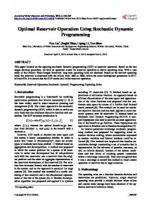
The problem addressed in this work is that of identifying an inventory replenishment policy for a product with a limited shelf life in a distribution network with serial configuration; the three echelons addressed are a single supplier, single distributor and single retailer as depicted in Figure 1. The retailer has a random stationary demand �� given by a discrete probability distribution. Based on retailer’s random demand, the distributor d orders a quantity ��� in period t from the supplier s, who in turn orders a quantity ��� in period t from his supplier. Distributor and supplier purchase products at a unit cost of � � and � � , respectively. The lead times for replenishing the supplier and distributor are assumed to be zero. Quantities are stored at both the supplier and distributor, whose capacity is assumed to be infinite. The products have a shelf life of M periods. Quantities reaching their shelf life are disposed of at a unit disposal cost w. Holding costs are incurred at both supplier and distributor and amount to ℎ � and ℎ� per unit per period, respectively. Furthermore, there is a fixed ordering cost k associated with each order. The inventory level at distributor and supplier in any period t is given by �� and �� , respectively. Any unmet demand is lost, and the initial � inventory levels at both supplier and distributor ( ,� � and ,� ) are zero. A predetermined service level α is targeted. The service level is calculated as the probability of no stock out during a replenishment cycle. The objective is to identify replenishment quantities for supplier ��� and distributor ��� per period t so as to minimize the total expected cost across the echelons and satisfy a service level constraint.
� �
���
Supplier ��
� �
���
Outdated items
Retailer
Distributor ��
��
Outdated items
Figure 1. Model description for period t.
3.2 Dynamic programming formulation of the problem Since the problem is characterized by making decision at each period based on the state of the system in previous stages and the decisions made, it lends itself to the dynamic programming approach. Having uncertain demand, the problem is modeled via stochastic dynamic programming. To this end the following elements have to be identified: the states, the decision variables, the contribution function, and the objective function. States are the inventory levels � at each echelon. The decisions made are the quantities ordered in each period t. The state transition function describes the inventory level in period t based on the inventory level in previous period (t-1) and the decision made in the current period t. The expected
3 Model development
2
MATEC Web of Conferences 68, 06006 (2016)
DOI: 10.1051/ matecconf/20166806006
ICIEA 2016 the product is disposed of at a wastage cost of $500 per unit. Ordering costs for supplier and distributor are $3,000. Unsold quantities are kept in inventory at a holding cost of $100 per unit per period. Initial inventory at distributor and supplier is assumed to be zero. From the cumulative probability it becomes evident, that it is necessary to have 2 or more units in stock to achieve a service level of 90%. Thus, orders are placed only, if at the beginning of the period less than 2 units are in stock. For this example quantities may be ordered in each period or aggregated and placed once at the beginning of the first period. The limited shelf life is considered by allowing to aggregate demand over only two periods, which is the product shelf life.
contribution to the objective function is comprised of fixed ordering cost, purchasing cost of quantities ��� and ��� , the expected holding and wastage costs. Backorders are not allowed in this model. The elements defining the stochastic programming model are described as follows: Stage (t): each stage presents a time period t, t=1,…,n, where n is the planning horizon. State (st): Inventory level at the beginning of period t. To meet a predefined service level, quantities on hand should satisfy the following equation: P(Idt ≥ 0)≥ α
(1)
Decision variables: the decision in stage t is the amount to order at the beginning of period t. Two decision variables are present ��� and ��� . Contribution function: the function providing the cost at stage t, given that the decision ��� and ��� is made. Optimal value function��� (�� )�: minimum expected cost from the beginning of period t to the end of the planning horizon, period n, given that the inventory on and is st at the beginning of period t. (�� (�� ) = ���∗ ) : optimal Optimal policy replenishment policy for period t, given that the on hand inventory is st. Transformation function: the change of inventory level (state) for the next stage based on the current state, stage, and decision. � ��
= ( �� + ��� − �� )�
4.2. Model solution The model is solved via backward induction. Starting at stage 2, the possible states (i.e. inventory levels) are 0, 1, 2, and 3. These represent the closing inventory, and are thus disposed of at the wastage cost. Thus the contribution function valuation for states 0 through 3 will be $0, $500, $1,000, and $1,500, respectively. For stage one, the possible states are 0, 1, 2, and 3, since there is only one stage to go and the maximum anticipated demand is 3 units. Based on the quantity on hand, a decision is made regarding how much to order. To achieve the required service level, orders are placed only if the quantity on hand is below 2 units. The order quantity is selected so as to increase the inventory level to 2 units. The consideration of the service level constraint helps decreasing the number of feasible scenarios to consider. For example, when the state is zero, the minimum amount to order should be 2, to satisfy the service level constraint. Similarly, if only one unit is on hand at the beginning of period t, at least one unit is to be ordered. To facilitate model solution, it is further assumed that the inventory levels at beginning of period t at supplier and distributors are identical. The associated costs of ordering, purchasing, inventory and valuation of previous stage are calculated for each scenario. These include cost data for both supplier and distributor. The expected cost of each decision made based on the current inventory level is the sum of the weighted total cost by the respective probability. A sample of the detailed calculations of stage 1 is displayed in Table 1. The calculations shown in the table display all the possible decisions if the state at the beginning of the period is 2. In such a case, two decisions are possible either to order nothing or order 1 unit. The order quantities are chosen so as to preserve the service level. After making the decision, the demand is revealed. And either 0, 1, or 2 units are sold. Note that since no backorders are allowed, any demand exceeding the available inventory level is lost. Here it is also assumed that the demand is equal to the amount sold. Accordingly, the state, i.e. inventory level at the end of the period may be calculated. The probability in the 4th column indicates the probability of satisfying the demand, i.e. probability of sales. It is derived from the given demand probabilities. All the cost elements of the distributor and supplier are calculated and
(2)
� = ( �� + ��� − ��� )� ��
(3)
Recurrence relation: the following equation indicates the optimal policy at stage t, given that the optimal policy at stage t+1 is known. �� (�� ) = min�� �
(4)
�[� � � � + �� ��� + ℎ� �� ] +� � � � + � � ��� + ℎ � �� + ���
� = 1, ⋯ , �
where � � and � � are binary variables which are equal to 1 if the order quantity is greater than zero, and E[.] denotes the expected value. Boundary conditions: (��� ) = 0.
4 Numerical illustration 4.1. Problem description The following example illustrates the application of the model to a serial multi-echelon distribution system. It is required to identify the order quantities of the supplier and distributor so as to satisfy the retailer’s demand with a service level (α) of 90% at minimum expected total cost. Demand is assumed to be a stationary discrete random variable with a known probability distribution. Demand values are 0, 1, 2, and 3 units with probabilities of 0.25, 0.4, 0.25, and 0.1, respectively. The planning horizon is 2 periods and the product life time is 2 periods, after which
3
MATEC Web of Conferences 68, 06006 (2016)
DOI: 10.1051/ matecconf/20166806006
ICIEA 2016 summed along with the previous stage valuation function f0. The expected contribution is the sum of the weighted total cost by the respective probability. Hence, for a given state of 2 units and a decision of no orders to place, the
expected cost is $740. From the previous calculations, the resulting optimal value function for stage 1 is attained as shown in Table 2.
Table 1. Sample of calculations made for stage 1.
2
��� = ��� 0
�� 0
2
0
2
0
2
1
state ��
0.25
�� 2
� � �� 0
�� ��� 0
ℎ� �� 200
1
0.4
1
0
0
100
0
2
0.35
0
0
0
0
0
0
0.25
3
3000
1000
300
3000
900
Prob.
� ��� 0
� � ��� 0
total cost
expected contribution
1400
740*
ℎ � �� 200
�� 1000
0
200
500
800
0
200
0
100
1500
200 9800
2
1
1
0.4
2
3000
1000
200
3000
900
100
1000
9200
2
1
2
0.25
1
3000
1000
100
3000
900
100
500
8600
2
1
3
0.1
0
3000
1000
0
3000
900
100
0
8000
probability of having the distributor ordering 3 units from the supplier in t=2 is 4/7=0.57. In this example the demand of the distributor in stage one is 0, 1, 2, and 3 with a probability of 0.51, 0.19, 0.19, and 0.11, respectively. Similarly, in stage 2, the probability of the distributor ordering 2 and 3 units is 0.43 and 0.57, respectively. Based on the probability and cost values, the corresponding expected total cost is calculated. The approach of backward induction is applied twice; one time for supplier and the second for the distributor. Total supply chain inventory cost is the sum cost of the optimal policy for each of the supplier and distributor. The results of the two approaches are compared in the following section.
For stage zero, only one state is possible, since we assumed an initial inventory level of zero. Decisions made are to order 0 through 3 units. The resulting optimal valuation function and the corresponding decision are $15,665 and 3 units, respectively. Table 2. Optimal value function and policy for stage 1.
States � ($) ���∗ (units)
0 10,340 2
1 8,440 1
9080
2 740 0
4.3. Experimentation In order to illustrate the effect of coordination between the different supply chain echelons, the problem has been solved via two approaches. The first approach is the one described in Section 4.2, where the replenishment policy is determined based on integrating the decision for both the distributor and supplier (Experiment 1). By adopting this approach it is assumed that both echelons order the same quantity. The second conducted experiment (Experiment 2) is solving the model sequentially for one echelon at a time disregarding the multi-echelon structure. More specifically, the order quantity of the distributor is determined based on the uncertain demand of the retailer; these quantities are used as demand for the supplier. Since the decision made regarding the order quantities at the distributor are based on expected values, it becomes necessary to determine the probability of the demand of the distributor. This is achieved by the following approximation. For each stage, all feasible decision alternatives for all the possible states are identified, and the relative frequency of each decision is determined. For example in stage 2, there is only one state, which is to have no quantities on hand. In such a case, either 2 or 3 units are to be ordered to achieve the required service level. Quantities sold will turn out to be 0, 1, or 2, if two units are ordered; and 0, 1, 2, or 3, if three units are ordered. Thus there are seven feasible decision alternatives. The decision of ordering 3 units occurs in four out of these seven alternatives. Hence, the
5 Results and discussion The results obtained from the dynamic programming model are presented in this section. Table 3 summarizes the results for the two experiments. Experiment 1 considers the joint economic replenishment, while Experiment 2 neglects the coordination between the supply chain echelons. Table 3. Summary of results.
Expected Cost ($)
Experiment 1 (with coordination) Experiment 2 (without coordination) % improvement via coordination
Distributor
Supplier
Total
9,275
6,390
15,665
8,355
10,729
19,084
-11.0%
40.4%
17.92%
The joint replenishment has a benefit of decreasing the total supply chain cost by 17.92%. Although an increase in cost at the distributor is noticeable, a larger decrease of cost at the supplier causes an overall
4
MATEC Web of Conferences 68, 06006 (2016)
DOI: 10.1051/ matecconf/20166806006
ICIEA 2016 improvement in the supply chain. This is in line with the findings in [1]. The current study has showed that the same results are attainable with the presence of uncertainty in demand. The main cost reduction for the supplier are due to decreasing the holding cost. In fact coordinating the replenishment policy shifts the inventory from the supplier to the distributor.
References 1. 2.
3.
6 Conclusions and future work
4. 5.
This work has presented a stochastic dynamic programming approach to manage inventory in a simple serial three-echelon supply chain for a product with limited shelf life. Demand is assumed to be a stationary discrete random variable with known probability distribution. The model has been solved via backward induction for a small size problem of two time periods and one retailer, one distributor and one supplier. Two experiments have been conducted to illustrate the impact of coordination on expected cost at each echelon and across the supply chain. Coordination has proved to decrease expected total cost across the supply chain. A cost savings of around 17% was attained due to coordination between the supplier and distributor. The current approach may be extended to study the effect of coordination in more complex network structures with multi-products. The further consideration of non-stationary and continuous demand will allow to approach the real life case.
6. 7. 8. 9. 10. 11. 12. 13. 14.
15.
5
C. H. Glock, Int. J. Prod. Econ., 135, 2, 671–686, (2012) I. Z. Karaesmen, A. Scheller–Wolf, and B. C.-K. Deniz, Planning Production and Inventories in the Extended Enterprise, 151 (2011) M. A. B. and A. Guiffrida, M. Y. Jaber, and M. Khan, Manag. Res. Rev., 38, 3, 283–298 (2015) R. Haijema, Int. J. Prod. Econ., 157, 158–169 (2014) U. Abdulwahab and M. I. M. Wahab, Comput. Ind. Eng., 78, 259–270 (2014) I. Konstantaras and K. Skouri, Math. Probl. Eng., (2009) S. K. Goyal and B. C. Giri, Eur. J. Oper. Res., 134, 1, 1–16 (2001) M. Bakker, J. Riezebos, and R. H. Teunter, Eur. J. Oper. Res., 221, 275–284 (2012) A T. Gümüs and A F. Güneri, Proc. Inst. Mech. Eng. Part B J. Eng. Manuf., 221, 1553–1570 (2007) H. Rau, M. Y. Wu, and H. M. Wee, Int. J. Prod. Econ., 86, 155–168 (2003) A. Shastri, S. R. Singh, D. Yadav, and S. Gupta, Procedia Technol., 10, 320–329 (2013) K. G. J. Pauls-Worm and E. M. T. Hendrix, Lect. Notes Comput. Sci. 9157, 397–412 (2015) C. L. Williams and B. E. Patuwo, Eur. J. Oper. Res., 116, 352–373 (1999) E. M. T. Hendrix, R. Haijema, R. Rossi, and K. G. J. Pauls-Worm, Comput. Sci. Its Appl. - ICCSA 2012, Pt III, 7335, 45–56 (2012) R. Rossi, IFAC Proc., 2021–2026 (2013)