Hindawi Publishing Corporation Abstract and Applied Analysis Volume 2014, Article ID 836895, 8 pages http://dx.doi.org/10.1155/2014/836895
Research Article Study on Support Vector Machine-Based Fault Detection in Tennessee Eastman Process Shen Yin,1 Xin Gao,1 Hamid Reza Karimi,2 and Xiangping Zhu1 1 2
College of Engineering, Bohai University, Liaoning 121013, China Department of Engineering, Faculty of Engineering and Science, University of Agder, 4898 Grimstad, Norway
Correspondence should be addressed to Xin Gao;
[email protected] Received 19 February 2014; Accepted 1 April 2014; Published 24 April 2014 Academic Editor: Hui Zhang Copyright © 2014 Shen Yin et al. This is an open access article distributed under the Creative Commons Attribution License, which permits unrestricted use, distribution, and reproduction in any medium, provided the original work is properly cited. This paper investigates the proficiency of support vector machine (SVM) using datasets generated by Tennessee Eastman process simulation for fault detection. Due to its excellent performance in generalization, the classification performance of SVM is satisfactory. SVM algorithm combined with kernel function has the nonlinear attribute and can better handle the case where samples and attributes are massive. In addition, with forehand optimizing the parameters using the cross-validation technique, SVM can produce high accuracy in fault detection. Therefore, there is no need to deal with original data or refer to other algorithms, making the classification problem simple to handle. In order to further illustrate the efficiency, an industrial benchmark of Tennessee Eastman (TE) process is utilized with the SVM algorithm and PLS algorithm, respectively. By comparing the indices of detection performance, the SVM technique shows superior fault detection ability to the PLS algorithm.
1. Introduction Fault detection in manufacture process aims at timely nosing out abnormal process behavior. Early fault detection of process makes the process safer, more efficient and more economical and guarantees the quality of products. Therefore, several statistical methods appeared for fault diagnosis and detection, such as artificial neural networks (ANN), fuzzy logic systems, genetic algorithms, principal component analysis (PCA), and more recently support vector machine (SVM) [1]. SVM has been extensively studied and has been used to construct data-driven modeling, classifying, and fault detection due to its better generalization ability and nonlinear classification ability [2–4]. On the other hand, since massive amounts of data produced in the industrial manufacturing process can be recorded and collected, the study of data-driven technique has become an active research field. It can benefit diverse communities including process engineering [5, 6]. Over the past few years, linear supervised classification technique, for example, K-nearest neighbor [7], PCA [8, 9], Fisher discriminant analysis [8], discriminant partial least squares (DPLS) [8–10], and nonlinear classification technique, for example, ANN [11] and SVM [12],
have been proposed and greatly improved [13, 14]. Moreover, several machine learning algorithms have been applied in real processes and simulation processes [15–17]; for example, the PCA algorithm is used to analyse product quality for a pilot plant [18], PLS and PCA are applied in chemical industry for process fault monitoring [19], and the key performance indicator prediction scheme is applied into an industrial hot strip mill in [20]. The SVM algorithm can improve the detection accuracy and it started to be used for fault detection. Now it has been extensively used to solve classification problems in many domains, for example, face, object and text detection and categorization, information and image retrieval, and so forth. The algorithm of support vector machine (SVM) is studied detailedly in this paper. SVM is a representative nonlinear technique and it is a potentially effective technique for classifying all kinds of datasets [21]. Fault detection can be considered as a special classification problem involved in model-based method [22] and data-based method, with the purpose to timely recognise faulty condition. With the help of cross-validation algorithm to optimise parameters, the performance of classification is greatly enhanced [23–25]. Then, to test the classification performance of SVM algorithm,
2
Abstract and Applied Analysis
a simulation model, the Tennessee Eastman process, is used for detecting fault, which has 52 variables representing the dynamics of the process [26]. In this simulation, original dataset is handled using SVM algorithm and it obtains satisfactory fault detection result. In the process of model building and test data classifying, no other theory is added, relatively decreasing the calculation time and reducing the computational burden. Compared with PLS algorithm, classifier based on SVM performs higher accuracy. Finally, using the SVM-based classifier with optimal parameters, faulty station of the process is detected. The paper is arranged as follows. The SVM classification algorithm, PLS algorithm, and cross-validation algorithm are introduced in the next section. Sections 3 and 4 present an application to Tennessee Eastman process simulator using SVM and PLS algorithms, respectively, and SVM-based fault detection outperforms that of PLS algorithm. Section 5 summarizes a conclusion.
2. Method Algorithms 2.1. Support Vector Machines Theory. Support vector machine (SVM) is a relatively new multivariate statistical approach and has become popular due to its preferable effect of classification and regression. SVM-based classifier has better generalization property because it is based on the structural risk minimization principle [27]. SVM algorithm has the nonlinear attribute; thus, it can deal with large feature spaces [28]. Due to the aforementioned two factors, SVM algorithm begins to be used in machine fault detection. The fundamental principle of SVM is separating dataset into two classes according to the hyperplane (a decision boundary) which should have maximum distance between support vectors in each class. Support vectors are representative data points and their increasing number may increase the complexity of problem [28, 29]. This thesis uses a binary classifier with dataset and the corresponding labels. Training dataset containing two classes is given in matrix 𝑋 with the form of 𝑚 × 𝑛 [6], in which 𝑚 represents the number of observe samples, while 𝑛 stands for the quantity of the observed variables. 𝑥𝑖 is denoted as a column vector to stand for the 𝑖th row of 𝑋. Each sample is assumed to be in a positive class or in a negative class. Besides, a column vector 𝑌 serves as the class label, containing two entries −1 and 1. Denote that 𝑦𝑖 = 1 is associated with one class and 𝑦𝑖 = −1 with the other class. If the training dataset is linearly separable, the SVM will try to separate it by a linear hyperplane: 𝑓 (𝑥) = ⟨𝑤, 𝑥⟩ + 𝑏 = 0,
(1)
where 𝑤 is an 𝑚-dimensional vector and 𝑏 is a scalar. The parameters 𝑤 and 𝑏 decide the separating hyperplane’s position and orientation. A separating hyperplane is considered to be optimal if it creates maximum distance between the closest vectors and the hyperplane. The closest points in each class are denoted as support vectors. If other points in the training set are removed, the calculated decision boundary remains the same one. That is to say the support
vectors contain all information in the dataset to define the hyperplane. The distance 𝑑 from a data point 𝑥𝑖 to the separating hyperplane is |⟨𝑤, 𝑥⟩ + 𝑏| . ‖𝑤‖
𝑑=
(2)
Vapink in 1995 put forward a canonical hyperplane [30], where 𝑤 and 𝑏 should satisfy min ⟨𝑤, 𝑥𝑖 ⟩ + 𝑏 = 1. (3) 𝑖 That is to say if the nearest point is taken to the hyperplane function, the result is constrained to be 1. This restriction on the parameters is to simplify the formation of problem. In a way, as for a training data 𝑥𝑖 , 𝑦𝑖 , the separating hyperplane of the above-mentioned form will become 𝑦𝑖 𝑓 (𝑥𝑖 ) = 𝑦𝑖 (⟨𝑤, 𝑥𝑖 ⟩ + 𝑏) ≥ 1,
𝑖 = 1, . . . , 𝑚.
(4)
The best separating hyperplane is the one that makes maximum distance from support vectors to decision boundary. The maximum distance is denoted as 𝜌. Consider 𝜌=
1 . ‖𝑤‖
(5)
Hence, as for linear separable data, the optimal separating hyperplane satisfies the following function: 1 min 𝜙 (𝑤) = ‖𝑤‖2 . 2
(6)
To solve the optimal problem equation (6) under the constrain of (4), define the Lagrangian to be 𝑚 1 ℓ (𝑤, 𝑏, 𝛼) = ‖𝑤‖2 − ∑𝛼𝑖 [𝑦𝑖 (⟨𝑤, 𝑥𝑖 ⟩ + 𝑏) − 1] , 2 𝑖=1
(7)
where 𝛼𝑖 is called Lagrangian multiplier. The Lagrangian should be maximised by choosing appropriate 𝛼𝑖 and should be minimised by 𝑤, 𝑏. Taking the noise in the data and the misclassification of hyperplane into consideration, the above function describing the separate hyperplane equation (4) is not accurate enough. To make the optimal separating boundary to be generalised, we reformulate the described function of the separate hyperplane: 𝑦𝑖 (⟨𝑤, 𝑥𝑖 ⟩ + 𝑏) ≥ 1 − 𝜉𝑖 ,
𝑖 = 𝑖 . . . , 𝑚.
(8)
where the variable 𝜉𝑖 represents a measure of distance from hyperplane to misclassified points and 𝜉𝑖 ≥ 0. To find the optimal generalised separating hyperplane, the following optimal problem should be solved: min 𝑤,𝑏
𝑚 1 ‖𝑤‖2 + 𝐶 ∑ 𝜉𝑖 2 𝑘=1
s.t. 𝑦𝑖 (⟨𝑤, 𝑥𝑖 ⟩ + 𝑏) ≥ 1 − 𝜉𝑖 , 𝜉𝑖 ≥ 0,
𝑖 = 𝑖 . . . , 𝑚,
(9)
Abstract and Applied Analysis
3
where the parameter 𝐶, a given value, is called error penalty. As for the above-mentioned data inseparable case, in order to simplify the optimal problem, define the Lagrangian to be ℓ (𝑤, 𝑏, 𝜉, 𝛼, 𝛾) =
𝑚 1 ‖𝑤‖2 + 𝐶∑𝜉𝑖 2 𝑖=1
Table 1: Formulation of Kernel functions. 𝐾(𝑥𝑖 , 𝑥𝑗 ) 𝑥𝑖𝑇 ⋅ 𝑥𝑗 𝑇 (𝛾𝑥𝑖 ⋅ 𝑥𝑗 + constant)𝑑
Kernel Linear Polynomial
𝑒−𝛾||𝑥𝑖 −𝑥𝑗 ||
Gaussian RBF functions
𝑚
𝑚
𝑖=1
𝑖=1
2
𝛾, constant and 𝑑 are kernel parameters.
− ∑𝛼𝑖 [𝑦𝑖 (⟨𝑤, 𝑥𝑖 ⟩ + 𝑏) − 1 + 𝜉𝑖 ] − ∑𝛾𝑖 𝜉𝑖 , (10) where 𝛼, 𝛾 are the Lagrangian multipliers. We consider the minimization problem as original, primal problem. Consider min 𝜃𝑝 (𝑤) = min max ℓ (𝑤, 𝑏, 𝜉, 𝛼, 𝛾) . 𝑤,𝑏,𝜉 𝛼,𝛾
𝑤,𝑏,𝜉
(11)
When satisfying the Kuhn-Tucker condition, then the primal problem is transformed to its dual problem, which is max 𝜃𝑑 (𝛼, 𝛾) = max min ℓ (𝑤, 𝑏, 𝜉, 𝛼, 𝛾) . 𝛼,𝛾
𝛼,𝛾 𝑤,𝑏,𝜉
(12)
Then, the task is minimizing ℓ in (10) by adjusting the value of 𝑤, 𝑏, 𝜉. At the optimal point, derivatives of ℓ should be zero. The saddle-point equation is as follows: 𝑚
𝜕ℓ = 0, 𝜕𝑤
⇒ ∑𝛼𝑖 𝑦𝑖 = 0
(13)
𝑖=1
𝑚
𝜕ℓ = 0, 𝜕𝑏
The classifier implementing the optimal separating hyperplane comes out in the following form: 𝑚
𝑓 (𝑥) = sgn ( ∑ 𝛼𝑖 𝑦𝑖 ⟨𝑥𝑖 , 𝑥𝑗 ⟩ + 𝑏) .
(19)
𝑖,𝑗=1
However, in some cases linear classifier is not suitable; for example, data is overlapped or cannot be linearly separated. Therefore, the input vectors should be projected into a higher dimensional feature space and there the data may be linearly classified more efficiently with the use of SVM algorithm. However, it may cause computational problem due to the large vectors and high dimensionality. The idea of using Kernel function enables the calculation performed in the original space instead of in the projected high dimensioned future space, avoiding the curse of dimensionality [27, 31]. Given a feature mapping 𝜙, we define the corresponding Kernel function to be 𝐾 (𝑥𝑖 , 𝑥𝑗 ) = ⟨𝜙 (𝑥𝑖 ) , 𝜙 (𝑥𝑗 )⟩ .
(20)
⇒ 𝑤 = ∑𝛼𝑖 𝑦𝑖 𝑥𝑖
(14)
Thus, the linear decision hyperplane in the high feature space is
⇒ 𝛼𝑖 + 𝛾𝑖 = 𝐶.
(15)
𝑓 (𝑥) = sgn ( ∑ 𝛼𝑖 𝑦𝑖 ⟨𝐾 (𝑥𝑖 , 𝑥𝑗 )⟩ + 𝑏) .
𝑖=1
𝜕ℓ = 0, 𝜕𝜉
𝑚
(21)
𝑖,𝑗=1
If we take (13), (14), and (15) back into (10), we can obtain the dual quadratic optimization problem [30, 31]: 𝑚 { 1𝑚 𝑚 } 𝑊 = max 𝛼 𝛼 𝑦 𝑦 ⟨𝑥 , 𝑥 ⟩ + 𝛼𝑘 } . max − ∑ ∑ ∑ (𝛼) 𝑖 𝑗 𝑖 𝑗 𝑖 𝑗 𝛼 𝛼 { 2 𝑘=1 { 𝑖=1𝑗=1 } (16)
Satisfying the constrains: 0 ≤ 𝛼𝑖 ≤ 𝐶,
𝑖 = 1 . . . , 𝑚,
𝑚
∑𝛼𝑖 𝑦𝑖 = 0.
(17)
𝑖=1
When solved the dual quadratic optimization problem shown in (16), the 𝛼𝑖 will be obtained. Then take a look back at (14) and describe the optimal 𝑤 using 𝛼𝑖 and the form of hyperplane can be changed to 𝑚
⟨𝑤, 𝑥𝑖 ⟩ + 𝑏 = ∑ 𝛼𝑖 𝑦𝑖 ⟨𝑥𝑖 , 𝑥𝑗 ⟩ + 𝑏. 𝑖,𝑗=1
(18)
𝐾(𝑥𝑖 , 𝑥𝑗 ) is inexpensive to calculate. Kernel function returns an inner production of vectors in the high feature space which is evaluated in the original space not in high feature space. The commonly used four Kernel functions are as shown in Table 1. 2.2. SVM Model Selection. SVM algorithm is a very effective data classifying technique, and building a model to detect fault based on SVM algorithm is not so complex. Training dataset and testing sets are usually involved when a classification is done. Besides, every instance in the training set contains two parts: one is target value (i.e., the class label) and the other is several attributes (i.e., observed variables). The basic process of using SVM algorithm to classify data is as follows: at first build a classifier based on the training set and then use it to predict the target value of the data in testing set where only the attributes are known. To construct a classifier model and figure out faulty data, the following procedure is used. (i) Transform data collected from real process to the format that SVM classifier can use.
4
Abstract and Applied Analysis (ii) Try a few kinds of Kernels and find out the best one; then search the optimal parameters for it. This thesis uses Gaussian RBF Kernel function and the optimal parameters are obtained by using the cross-validation algorithm. (iii) Use the optimal parameters and appropriate Kernel function to build a classifier. (iv) Take testing data into the constructed classifier and do a test. As a result the faulty data will be figured out and in this way the faulty station can be detected.
2.3. PLS for Fault Detection. The PLS algorithm is introduced by Dayal and Macgregor [32] due to its simplicity and the lesser computational effort when dealing with the process monitoring with large data. In this technique, we also denote training data in the form of 𝑚 × 𝑛 matrix 𝑋, in which 𝑚 represents the number of observed samples, while 𝑛 is the quantity of the attributes and 𝑌 ∈ R𝑚×1 . The PLS algorithm projects the matrix 𝑋 into a low dimensional space with latent variables, and 𝑌 can be constructed by these latent variables. The construct model is as follows: 𝐴
2.2.1. RBF Kernel. Which kind of Kernel functions to use is significant, because it decides the feature space where training data is classified. Theoretically, the Kernel function is considered to be better if it can provide higher upper bound on the VC dimension. However, it requires evaluating the hypersphere enclosing all data in the nonlinear feature space, which is difficult to accomplish. Among the commonly used Kernel functions for the SVM algorithm, the RBF Kernel is preferable according to practical experience. Kernel function can nonlinearly project original input data to a higher dimensional space; thus, SVM equipped with Kernel function is able to deal with the case where the input data cannot be linearly separated. Generally speaking, the RBF Kernel is the first choice for the following two reasons. Firstly, linear Kernel is a special RBF Kernel—when the parameter 𝐶 is adjusted to a certain value, linear Kernel behaves similarly to RBF Kernel and so it is the sigmoid Kernel at some parameters. Secondly, the RBF Kernel brings fewer computational costs and fewer hyperparameters [23]. 2.2.2. Cross-Validation. When using an RBF Kernel function, it needs appropriate parameters to make sure that the classifier accurately predicts unknown data. It is not known beforehand what the best parameter values are; nevertheless, the optimal parameter searching can be accomplished using cross-validation algorithm [23]. The cross-validation algorithm is a model validation method which is used to evaluate the accuracy of a predictive model. The goal of cross-validation is to give an insight on how the model generalizes to an independent dataset (i.e., an unknown dataset) by defining a dataset in the training phase to test the model. In the process of 𝑘-fold cross-validation, original training set is randomly divided into k equal size parts. Sequentially, one subset is used as the testing dataset to test the predictive model and the rest of 𝑘 − 1 subsets are combined as the training dataset. The aforementioned validation process should be repeated 𝑘 times in all, with every subset performed as testing data once. Using the 𝑘 results, the predictive result of the model is produced and it is the overall misclassification rate across all testing sets. This thesis uses 5-fold cross-validation algorithm to find out the overall misclassification rate across all testing sets. The cross-validation process should be performed many times to pick out the parameters which make the overall misclassification minimise. In this way, the optimal parameters are found and the classifier can obtain the best accuracy rate.
𝑋 = 𝑇𝑃𝑇 + 𝐸 = ∑𝑡𝑖 𝑝𝑖𝑇 + 𝐸, 𝑖=1
𝑇
𝑌 = 𝑇𝑄 + 𝐹 =
(22)
𝐴
∑𝑡𝑖 𝑞𝑖𝑇 𝑖=1
+ 𝐹,
where 𝑇 = [𝑡1 , . . . 𝑡𝐴 ] is the score matrix of 𝑋. 𝑃 = [𝑝1 , . . . 𝑝𝐴 ] and 𝑄 = [𝑞1 , . . . 𝑞𝐴 ] are the loading matrix of 𝑋 and 𝑌, respectively. The latent variables 𝑡𝑖 ∈ 𝑇 (𝑖 = 1, . . . , 𝐴) can be directly calculated from 𝑋 by 𝑡𝑖 = 𝑋𝑟𝑖 ; 𝑅 = [𝑟1 , . . . 𝑟𝐴] and 𝑟𝑖 are calculated by the following: 𝑟1 = 𝑤1 , 𝑇 𝑤𝑖 𝑟𝑖−1 , 𝑟𝑖 = 𝑤𝑖 − 𝑝1𝑇 𝑤𝑖 𝑟1 − 𝑝𝑖−1
𝑖 = 2, . . . , 𝐴,
(23)
where the 𝑤𝑖 (𝑖 = 1, . . . , 𝐴) is the weight vector of the 𝑖th deflated 𝑋. PLS decomposes 𝑋 into two parts: ̃ 𝑥 = 𝑥̂ + 𝑥, 𝑥̂ = 𝑃𝑅𝑇 𝑥 ∈ 𝑆𝑥̂ ,
(24)
𝑥̃ = (𝐼 − 𝑃𝑅𝑇 ) 𝑥 ∈ 𝑆𝑥̃ . Usually, 𝑇2 statistic is used to detect abnormalities and the calculation method is −1
𝑇𝑇 𝑇 𝑇 = 𝑥 𝑅( ) 𝑅𝑇 𝑥. 𝑛−1 2
𝑇
(25)
With a given confidence level 𝛼, the threshold for 𝑇2 will be calculated by the following: 𝐽th,𝑇2 =
𝐴 (𝑛2 − 1) 𝑛 (𝑛 − 𝐴)
𝐹𝑙,𝑛−𝑙,𝛼 ,
(26)
where 𝐹𝑙,𝑛−𝑙,𝛼 represents 𝐹-distribution with l and 𝑁 − 1 degrees of freedom and its confidence level is 𝛼. If 𝑇2 are all less than their corresponding thresholds, the process is out of fault [32].
3. Simulation 3.1. Tennessee Eastman Process. The Tennessee Eastman process (TE process) is a simulation model of a practical industrial process. The simulation model is very suitable for researching on process control technology and also applicable
Abstract and Applied Analysis
5 FI 8
1
Condenser
JI
CWS
FI
2
D
XC
PI
LI
TI CWS
XA Analyzer
XD
FI
XF
XG
FI 10
XH Vap/liq separator
TI TI TI
12
CWR XD
FI
LI
Stm Reactor Cond
C
XE
Stripper 6
XE
FI
XD XF
PI
XB XC
XB
PI
CWR
3
Purge XA
5
TI
7
FI E
Compressor LI
SC
9
Analyzer
A
FI
FI 4
11
Analyzer
FI
XE XF XG XH Product
Figure 1: The flowsheet of TE process.
for other kinds of control issues. Figure 1 shows the flowsheet of TE process. The TE process consists of five major parts: the reactor, the product condenser, a vapor-liquid separator, a recycle compressor, and a product stripper to help accomplish reactor, separator, and recycle arrangement. More details can be found in [33, 34].
the PLS algorithm using the dataset generated by TE process simulator. For SVM classifier, the RBF Kernel is used and the related parameters will be set ahead according to the result of cross-validation to make sure of the classifier’s high accuracy. In the comparison, the performance is measured by fault detection rates.
3.2. Simulated Data Intro. The TE process is a plant-wide closed-loop control structure. The simulated process can produce normal operating condition as well as 21 faulty conditions and generate simulated data at a sampling interval of 3 min. For each case (no matter normal or faulty condition), two sets of data are produced, training datasets and testing datasets. The training sets are used to construct statistical predictive model and the testing datasets are used to estimate the accuracy of the built classifier. In training sets, the normal dataset contains 500 observation samples, while each faulty dataset contains 480 observation samples. As for testing data, each dataset (both normal and faulty conditions) consists of 960 observations. In the faulty condition, faulty information emerges 8h later since the TE process is turned on. That is to say, in each faulty condition, the former 160 samples are shown normally, while the remaining 800 instances are shown really faulty and should be detected. Every observation sample contains 52 variables which consists of 22 process measure variables, 19 component measure variables, and 12 control variables. All the datasets used in this paper can be found in [1]. In the following section, the fault detection result of SVMbased classifier will be compared with the one based on
4. Result and Discussion TE process simulator can generate 22 types of conditions, containing the normal condition and 21 kinds of programmed faults caused by various known disturbances in the process. Once fault is added, all variables will be affected and some changes will emerge. According to Chiang et al. [8] and Zhang [18] detection for faults 3, 9, 15, and 21 is very difficult for there are not any observable changes in the means, variance, or the peak time. Therefore, these four faults always cannot be detected by any statistics technique; thus, the four faults are not analysed in this paper. The information of all the faults is presented in Table 2. In order to profoundly test the detection effect of the classifier based on theory of SVM, the SVM algorithm and PLS algorithm are applied to the TE process, respectively. As for SVM classifier, all faults data are by turns combined with the normal condition data as the dataset for binary classifier. After models are built by training data, we use testing data to evaluate the prediction result through the following common indices: accuracy (Acc) and fault detection rate (FDR) [35]. Then the detection result for each fault is shown in Table 3. Table 4 represents the detection result using PLS technique.
6
Abstract and Applied Analysis Table 2: Descriptions of 21 faults in TE process.
Number IDV0 IDV1 IDV2 IDV4 IDV5 IDV6 IDV7 IDV8 IDV10 IDV11 IDV12 IDV13 IDV14 IDV16 IDV17 IDV18 IDV19 IDV20
Table 4: Results of faults detection using PLS algorithm.
Fault description Normal 𝐴/𝐶 feed ratio, 𝐵 composition constant B composition, 𝐴/𝐶 ratio constant Reactor cooling water inlet temperature Condenser cooling water inlet temperature A feed loss (stream 1) C header pressure loss-reduced availability (stream 4) A, B, and C feed composition (stream 4) C feed temperature (stream 4) Reactor cooling water inlet temperature Condenser cooling water inlet temperature Reaction kinetics Reactor cooling water valve Unknown Unknown Unknown Unknown Unknown
Fault IDV1 IDV2 IDV4 IDV5 IDV6 IDV7 IDV8 IDV10 IDV11 IDV12 IDV13 IDV14 IDV16 IDV17 IDV18 IDV19 IDV20
FDR (%) 𝑇𝑥̂2 99.37 98.75 0.63 16.65 99 29.16 89.86 18.15 2.63 76.85 92.62 2.25 9.39 4.88 87.48 0.38 18.4
𝑇𝑥̃2 99.62 98.12 97.25 30.04 100 100 96.87 43.55 68.84 98.37 94.99 100 29.41 91.74 89.86 15.14 50.44
Table 3: Results of faults detection with one against one classifier. Fault IDV1 IDV2 IDV4 IDV5 IDV6 IDV7 IDV8 IDV10 IDV11 IDV12 IDV13 IDV14 IDV16 IDV17 IDV18 IDV19 IDV20
Acc (%) 98.44 98.12 99.9 91.98 66.77 99.58 96.35 77.71 73.02 97.4 93.33 89.06 80.73 83.85 90.1 74.48 77.5
FDR (%) 99.5 98.12 99.88 90.75 60.13 98.91 96 81 80.25 97.75 92.5 91 89.38 81.63 89.5 85.88 80.5
Consider (i)
Acc =
the quantity of data correctly predicated the quantity of all data × 100%
(ii)
FDR =
number of faulty data correctly predicated number of all faulty data × 100%. (27)
Figure 2 shows the predicted label 𝑦 using three classifiers with the training and testing data respectively come from normal condition and fault 1, normal condition and fault 2, and normal condition and fault 4. The first 160th test, the process shows normally and 𝑦 should be −1. The fault information appears at the moment of 161st sample-taken and the label y should be 1 since then. From Figure 2, we can see that the SVM classifier’s prediction result for most of the time is right. In addition, Table 3 presents detailed detection indices of these 21 SVM classifiers. It is worth mentioning that the hyperparameters of the classifiers are all optimized beforehand. Without the optimization of classifier parameter, the predicted effect will not be so good. Moreover, the index accuracy will be 16.77% when using classifier’s default parameters to detect fault 1. Table 4 shows the detailed indices using PLS technique to detect faults. It can be seen that the SVM classifiers with optimal hyperparameters are mostly able to detect the faulty data, and the accuracy is higher than that given by using PLS algorithm. Therefore, the SVM algorithm has a better performance of fault detection. To further test the predictive ability of the SVM classifier, that is, the detective ability of fault in the TE process, we use normal condition data combined with three faulty condition datasets (fault 1, fault 2, fault 4) as the training data to construct a classification model and then used corresponding test data as testing data to observe the classification result. As shown in Table 5, the detection indices are also good though the computing time is a little longer with the same compute facility. Thus the SVM algorithm can perform satisfactorily on the original dataset containing 52 attributes without any transformation. In this way, in real process, with advanced compute facility, we can train normal data and all faults data to build a classifier. Once the fault label is figured out, the fault in process is detected.
Abstract and Applied Analysis
7
SVM(one versus one) on test data y (0 versus 2)
y (0 versus 4)
0
−2
0
200
400
600
SVM(one versus one) on test data
2
2
800
1000
0
−2
0
200
400
(a)
600
800
1000
(b) SVM(one versus one) on test data
y (0 versus 4)
2
0
−2
0
200
400
600
800
1000
(c)
Figure 2: Classification results for the testing dataset by the SVM-based classifier with optimal parameters. The value 𝑦 = −1 represents at the sample-taken moment that the process is in normal condition, while 𝑦 = 1 stands for faulty condition. The top plot is the classification result between normal condition and fault 1, the middle one is the result between normal condition and fault 2, and the last plot is result between normal condition and fault 4. In the simulation of fault condition, the fault information appears from the moment of 161th sample-taken and it is pointed out by red line.
Table 5: Results of faults detection with one against all classifier. Test description 0 versus 1, 2 0 versus 1, 2 0 versus 1, 2 0 versus 1, 2, 4 0 versus 1, 2, 4 0 versus 1, 2, 4 0 versus 1, 2, 4
Test data IDV1 test data IDV2 test data IDV0 test data IDV1 test data IDV2 test data IDV4 test data IDV0 test data
Acc (%) 98.02 95.83 83.44 96.46 95 96.98 79.62
FDR (%) 99.62 98.5 99.75 98.88 100
when the number of samples or attributes is very large. By comparing detection performance with classifier based on the PLS algorithm, the classifier based on SVM algorithm with Kernel function shows superior accuracy rate. In addition, parameter optimization beforehand plays a great role in improving the effectiveness of classification. It also simplifies the problem and by using no other technique relatively decreases the computational load to reach a satisfactory classification result as well.
Conflict of Interests From the above-shown result of fault detection on TE process, we can conclude that the classifier based on SVM algorithm is of good predictive ability. In addition, there are two facts that should be mentioned. First, before detecting normal condition or faulty condition, we have used the technique of cross-validation to optimize classifier’s hyperparameters. Therefore, the performance of classifier could be the best. Second, the classification on TE process based on SVM algorithm performs satisfactorily without any other process, for example, foregoing data dealing process and attributes selection. And this feature makes the SVM classifier easy to be built. Besides, the calculation and calculate time is relatively small since the algorithms used are fewer.
5. Conclusion TE process, a benchmark chemical engineering model, is used in this paper for fault detection. It can be found that the fault detection ability of the classifier based on SVM algorithm using the TE process’s original data is satisfactory and this indicates the advantage of using nonlinear classification
The authors declare that there is no conflict of interests regarding the publication of this paper.
References [1] S. Yin, Data-driven design of fault diagnosis systems [Ph.D. dissertation], University of Duisburg-Essen, 2012. [2] V. N. Vapnik, The Nature of Statistical Learning Theory, Springer, New York, NY, USA, 1995. [3] B. E. Boser, I. M. Guyon, and V. N. Vapnik, “Training algorithm for optimal margin classifiers,” in Proceedings of the 5h Annual ACM Workshop on Computational Learning Theory, pp. 144– 152, New York, NY, USA, July 1992. [4] C. Cortes and V. Vapnik, “Support-vector networks,” Machine Learning, vol. 20, no. 3, pp. 273–297, 1995. [5] A. Kulkarni, V. K. Jayaraman, and B. D. Kulkarni, “Support vector classification with parameter tuning assisted by agentbased technique,” Computers and Chemical Engineering, vol. 28, no. 3, pp. 311–318, 2004. [6] L. H. Chiang, M. E. Kotanchek, and A. K. Kordon, “Fault diagnosis based on Fisher discriminant analysis and support
8
[7] [8]
[9]
[10]
[11] [12]
[13]
[14]
[15]
[16]
[17]
[18]
[19]
[20]
[21]
[22]
[23]
[24]
Abstract and Applied Analysis vector machines,” Computers and Chemical Engineering, vol. 28, no. 8, pp. 1389–1401, 2003. K. R. Beebe, R. J. Pell, and M. B. Seasholtz, Chemometrics: A Practical Guide, Wiley, New York, NY, USA, 1998. L. H. Chiang, E. L. Russell, and R. D. Braatz, Fault Detection and Diagnosis in Industrial Systems, Springer, New York, NY, USA, 2001. A. Raich and A. C ¸ inar, “Statistical process monitoring and disturbance diagnosis in multivariable continuous processes,” AIChE Journal, vol. 42, no. 4, pp. 995–1009, 1996. L. H. Chiang, E. L. Russell, and R. D. Braatz, “Fault diagnosis in chemical processes using Fisher discriminant analysis, discriminant partial least squares, and principal component analysis,” Chemometrics and Intelligent Laboratory Systems, vol. 50, no. 2, pp. 243–252, 2000. D. R. Baughman, Neural Networks in Bioprocessing and Chemical Engineering, Academic Press, New York, NY, USA, 1995. T. Hastie, R. Tibshirani, and J. Friedman, The Elements of Statistical Learning: Data Mining, Inference, and Prediction, Springer, New York, NY, USA, 2009. A. S. Naik, S. Yin, S. X. Ding, and P. Zhang, “Recursive identification algorithms to design fault detection systems,” Journal of Process Control, vol. 20, no. 8, pp. 957–965, 2010. S. X. Ding, S. Yin, P. Zhang, E. L. Ding, and A. Naik, “An approach to data-driven adaptive residual generator design and implementation,” in Proceedings of the 7th IFAC Symposium on Fault Detection, Supervision and Safety of Technical Processes, pp. 941–946, Barcelona, Spain, July 2009. S. Ding, P. Zhang, S. Yin, and E. Ding, “An integrated design framework of fault-tolerant wireless networked control systems for industrial automatic control applications,” IEEE Transactions on Industrial Informatics, vol. 9, no. 1, pp. 462–471, 2013. H. Zhang, Y. Shi, and A. Mehr, “On 𝐻∞ filtering for discretetime takagi-sugeno fuzzy systems,” IEEE Transactions on Fuzzy Systems, vol. 20, no. 2, pp. 396–401, 2012. H. Zhang and Y. Shi, “Parameter dependent 𝐻∞ filtering for linear time-varying systems,” Journal of Dynamic Systems, Measurement, and Control, vol. 135, no. 2, Article ID 0210067, 7 pages, 2012. Y. W. Zhang, “Enhanced statistical analysis of nonlinear process using KPCA, KICA and SVM,” Chemical Engineering Science, vol. 64, pp. 800–801, 2009. M. Misra, H. H. Yue, S. J. Qin, and C. Ling, “Multivariate process monitoring and fault diagnosis by multi-scale PCA,” Computers and Chemical Engineering, vol. 26, no. 9, pp. 1281–1293, 2002. S. Ding, S. Yin, K. Peng, H. Hao, and B. Shen, “A novel scheme for key performance indicator prediction and diagnosis with application to an industrial hot strip mill,” IEEE Transactions on Industrial Informatics, vol. 9, no. 4, pp. 2239–2247, 2013. B. Scholkopf and A. J. Smola, Learning with Kernels, Support Vector Machines, Regularization, Optimization, and Beyond, MIT Press, New York, NY, USA, 2002. N. F. Thornhill and A. Horch, “Advances and new directions in plant-wide disturbance detection and diagnosis,” Control Engineering Practice, vol. 15, no. 10, pp. 1196–1206, 2007. C. W. Hsu, C. C. Chang, and C. Lin, A Practical Guide to Support Vector Classification, Department of Computer Science, National Taiwan University, 2010. T. Hastie, R. Tibshirani, and J. Friedman, The Elements of Statistical Learning, Springer, New York, NY, USA, 2001.
[25] J. C. Lagarias, J. A. Reeds, M. H. Wright, and P. E. Wright, “Convergence properties of the Nelder-Mead simplex method in low dimensions,” SIAM Journal on Optimization, vol. 9, no. 1, pp. 112–147, 1998. [26] A. Kulkarni, V. K. Jayaraman, and B. D. Kulkarni, “Knowledge incorporated support vector machines to detect faults in Tennessee Eastman process,” Computers and Chemical Engineering, vol. 29, no. 10, pp. 2128–2133, 2005. [27] S. R. Gunn, Support Vector Machines for Classification and Regression, Faculty of Engineering, Science and Mathematics School of Electronics and Computer Science, 1998. [28] A. Widodo and B. Yang, “Support vector machine in machine condition monitoring and fault diagnosis,” Mechanical Systems and Signal Processing, vol. 21, no. 6, pp. 2560–2574, 2007. [29] C. J. C. Burges, “A tutorial on support vector machines for pattern recognition,” Data Mining and Knowledge Discovery, vol. 2, no. 2, pp. 121–167, 1998. [30] V. N. Vapnik, Statistical Learning Theory, John Wiley & Sons, New York, NY, USA, 1998. [31] N. Cristianini and J. Shawe-Taylor, An Introduction to Support Vector Machines, Cambridge University Press, 2000. [32] B. S. Dayal and J. F. Macgregor, “Improved PLS algorithms,” Journal of Chemometrics, vol. 11, no. 1, pp. 73–85, 1997. [33] P. R. Lyman and C. Georgakis, “Plant-wide control of the Tennessee Eastman problem,” Computers and Chemical Engineering, vol. 19, no. 3, pp. 321–331, 1995. [34] J. J. Downs and E. F. Vogel, “A plant-wide industrial process control problem,” Computers and Chemical Engineering, vol. 17, no. 3, pp. 245–255, 1993. [35] S. Yin, S. X. Ding, A. Haghani, H. Hao, and P. Zhang, “A comparison study of basic data-driven fault diagnosis and process monitoring methods on the benchmark tennessee eastman process,” Journal of Process Control, vol. 22, pp. 1567– 1581, 2012.
Advances in
Operations Research Hindawi Publishing Corporation http://www.hindawi.com
Volume 2014
Advances in
Decision Sciences Hindawi Publishing Corporation http://www.hindawi.com
Volume 2014
Journal of
Applied Mathematics
Algebra
Hindawi Publishing Corporation http://www.hindawi.com
Hindawi Publishing Corporation http://www.hindawi.com
Volume 2014
Journal of
Probability and Statistics Volume 2014
The Scientific World Journal Hindawi Publishing Corporation http://www.hindawi.com
Hindawi Publishing Corporation http://www.hindawi.com
Volume 2014
International Journal of
Differential Equations Hindawi Publishing Corporation http://www.hindawi.com
Volume 2014
Volume 2014
Submit your manuscripts at http://www.hindawi.com International Journal of
Advances in
Combinatorics Hindawi Publishing Corporation http://www.hindawi.com
Mathematical Physics Hindawi Publishing Corporation http://www.hindawi.com
Volume 2014
Journal of
Complex Analysis Hindawi Publishing Corporation http://www.hindawi.com
Volume 2014
International Journal of Mathematics and Mathematical Sciences
Mathematical Problems in Engineering
Journal of
Mathematics Hindawi Publishing Corporation http://www.hindawi.com
Volume 2014
Hindawi Publishing Corporation http://www.hindawi.com
Volume 2014
Volume 2014
Hindawi Publishing Corporation http://www.hindawi.com
Volume 2014
Discrete Mathematics
Journal of
Volume 2014
Hindawi Publishing Corporation http://www.hindawi.com
Discrete Dynamics in Nature and Society
Journal of
Function Spaces Hindawi Publishing Corporation http://www.hindawi.com
Abstract and Applied Analysis
Volume 2014
Hindawi Publishing Corporation http://www.hindawi.com
Volume 2014
Hindawi Publishing Corporation http://www.hindawi.com
Volume 2014
International Journal of
Journal of
Stochastic Analysis
Optimization
Hindawi Publishing Corporation http://www.hindawi.com
Hindawi Publishing Corporation http://www.hindawi.com
Volume 2014
Volume 2014