Sub-Space Clustering, Inter-Clustering Results Association & Anomaly

Sub-Space Clustering, Inter-Clustering Results Association & Anomaly Correlation for Unsupervised Network Anomaly Detection Johan Mazel∗† , Pedro Casas∗† , Yann Labit∗† and Philippe Owezarski∗† ∗ CNRS;

† Universit´e

LAAS; 7 avenue du colonel Roche, F-31077 Toulouse Cedex 4, France de Toulouse; UPS, INSA, INP, ISAE ; UT1, UTM, LAAS; F-31077 Toulouse Cedex 4, France

Abstract—Network anomaly detection is a critical aspect of network management for instance for QoS, security, etc. The continuous arising of new anomalies and attacks create a continuous challenge to cope with events that put the network integrity at risk. Most network anomaly detection systems proposed so far employ a supervised strategy to accomplish the task, using either signature-based detection methods or supervised-learning techniques. However, both approaches present major limitations: the former fails to detect and characterize unknown anomalies (letting the network unprotected for long periods) , the latter requires training and labelled traffic, which is difficult and expensive to produce. Such limitations impose a serious bottleneck to the previously presented problem. We introduce an unsupervised approach to detect and characterize network anomalies, without relying on signatures, statistical training, or labelled traffic, which represents a significant step towards the autonomy of networks. Unsupervised detection is accomplished by means of robust dataclustering techniques, combining Sub-Space clustering with Evidence Accumulation or Inter-Clustering Results Association, to blindly identify anomalies in traffic flows. Correlating the results of the unsupervised detection is also performed for improving the detection robustness. Characterization is achieved by building efficient filtering rules to describe a detected anomaly. The detection and characterization performances of the unsupervised approach are evaluated on real network traffic. Index Terms—Unsupervised Anomaly Detection & Characterization, Clustering, Clusters Isolation, Outliers Detection, Filtering Rules, Anomaly Correlation.

I. I NTRODUCTION Network anomaly detection has become a vital component of any network in today’s Internet. Ranging from nonmalicious unexpected events such as flash-crowds and failures, to network attacks such as denials-of-service and network scans, network traffic anomalies can have serious detrimental effects on the performance and integrity of the network. The principal challenge in automatically detecting and characterizing traffic anomalies is that these are moving targets. It is difficult to precisely and permanently define the set of possible anomalies that may arise, especially in the case of network attacks, because new attacks as well as new variants of already known attacks are continuously emerging. A general anomaly detection system should therefore be able to detect a wide range of anomalies with diverse structures, using the least amount of previous knowledge and information, ideally none. The problem of network anomaly detection has been extensively studied during the last decade. Two different ap-

proaches are by far dominant in current research literature and commercial detection systems: signature-based detection and supervised-learning-based detection. Both approaches require some kind of guidance to work, hence they are generally referred to as supervised-detection approaches. Signaturebased detection systems are highly effective to detect those anomalies which are programmed to alert on. When a new anomaly is discovered, generally after its occurrence, the associated signature is coded by human experts, which is then used to detect a new occurrence of the same anomaly. Such a detection approach is powerful and very easy to understand, because the operator can directly relate the detected anomaly to its specific signature. However, these systems cannot defend the network against new attacks, simply because they cannot recognize what they do not know. Furthermore, building new signatures is expensive, as it involves manual inspection by human experts. On the other hand, supervised-learning-based detection uses labelled traffic data to train a baseline model for normaloperation traffic, detecting anomalies as patterns that deviate from this model. Such methods can detect new kinds of anomalies and network attacks not seen before, because they will naturally deviate from the baseline. Nevertheless, supervised-learning requires training, which is timeconsuming and depends on the availability of purely anomalyfree traffic data-sets. Labelling traffic as anomaly-free is expensive and hard to achieve in practice, since it is difficult to guarantee that no anomalies are hidden inside the collected traffic. Additionally, it is not easy to maintain an accurate and up-to-date model for anomaly-free traffic, particularly when new services and applications are constantly emerging. We think that modern anomaly detection systems should not rely on previously acquired knowledge and be able to autonomously detect and characterize traffic deviating from normal-operation one. Autonomous security is a strong requirement in current networks. It is not acceptable to still rely on a human hand made analysis of anomalies and attacks for defining suited countermeasures. Such a hand made process is slow, inefficient, costly and lets the network unprotected for several days in general. The current business process in network security is not fulfilling network requirements in terms of fully efficient security. We therefore proposed a completely unsupervised method to detect and characterize

l

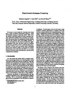
network anomalies, without relying on signatures, training, or labelled traffic of any kind. It adds to network (e.g. routers) or security components, thanks to unsupervised learning, some analysis and decision making capabilities for limiting the need of a human operator. This aims at making decision very fast, and configure efficiently and autonomously actual security devices (IDS, firewall, ...) as soon as a new anomaly or attack is encountered. A first version of the unsupervised anomaly detection method was initially proposed in [1]. It relies on the use of sub-space clustering and Evidence Accumulation. This first proposed approach permits to detect both well-known as well as completely unknown anomalies, and to automatically produce easy-to-interpret signatures that characterize them. In this paper, a new augmented version of this previous proposal is presented. The global objectives are similar. Nevertheless, it aims at increasing robustness and correctness of the decision making process by integrating new techniques as Inter-Clustering Result Association (ICRA) and Anomaly Correlation. Figure 1 depicts the high-level structure of our approach and its steps. It depicts both the techniques presented in previous papers (that will be nevertheless shortly presented in this one for making the paper self contained and understandable without referring to this previous publication) as well as the new ones recently integrated and which constitutes the new contribution: ICRA and Anomaly Correlation. Figure 1 serves all along this paper, and will be further described in the following sections. The remainder of the paper is organized as follows. Section II presents a very brief state of the art in the supervised and unsupervised anomaly detection fields, additionally describing our main contributions. Section III presents an indepth description of the clustering techniques and detection algorithms that we use. Section IV presents the anomaly correlation technique that improves the anomaly extraction phase. Section V presents the automatic anomaly characterization algorithm, which builds easy-to-interpret signatures for the detected anomalies. Section VI evaluates the computational time of the unsupervised detection approach, considering the parallelization of the clustering algorithms. Section VII presents a simple validation of our proposals, discovering and characterizing several anomalies in real network traffic from the MAWI trace repository [2]. Finally, section VIII concludes this paper. II. R ELATED W ORK The problem of network anomaly detection has been extensively studied during the last decade. Traditional approaches analyze statistical variations of traffic volume metrics (e.g., number of bytes, packets, or flows) and/or other specific traffic features (e.g. distribution of IP addresses and ports), using either single-link measurements or network-wide data. A non-exhaustive list of methods includes the use of signal processing techniques (e.g., ARIMA, wavelets) on single-link traffic measurements [3], [4], PCA [5], [6] and Kalman filters [7] for network-wide anomaly detection, and Sketches applied to IP-flows [8], [9].

Zt1

Network Traffic Capturing

Multi Resolution Flow Aggregation

X

l

Zt2

X2

. . . . .

Y 1 2 3 4

XN

Density-based Clusteing

. . . . .

P1

F (Zti )

Computation of Features

SSC

X1

Change Detection l

l Zt9

P2

Fig. 1.

Network Anomalies

Detection Threshold

PN

(EA || ICRA) + Anomaly Correlation

Th n

High-level description of our approach.

The URCA tool [10] has an hybrid approach which relies on both signatures and supervised learning. This tool uses as input the result of any anomaly detection system. It is able to classify anomalies by associating them with previously manually built signatures through hierarchical clustering. However, if the anomaly detection algorithm used detects an anomaly which is different from every built-in signature, this system is unable to classify or characterize the considered unknown anomaly. Our proposal falls within the unsupervised anomaly detection domain. Most work has been devoted to the Intrusion Detection field, focused on the well known KDD’99 data-set. The vast majority of the unsupervised detection schemes proposed in the literature are based on clustering and outliers detection, being [11]–[13] some relevant examples. In [11], authors use a single-linkage hierarchical clustering method to cluster data from the KDD’99 data-set, based on the standard Euclidean distance for inter-pattern similarity. Clusters are considered as normal-operation activity, and patterns lying outside a cluster are flagged as anomalies. Based on the same ideas, [12] reports improved results in the same data-set, using three different clustering algorithms: Fixed-Width clustering, an optimized version of k-NN, and one class SVM. Finally, [13] presents a combined density-grid-based clustering algorithm to improve computational complexity, obtaining similar detection results. III. U NSUPERVISED A NOMALY D ETECTION The algorithm runs in three consecutive stages. Firstly, multi-resolution flow aggregation is applied on the traffic in order to build several simple metrics such as number of bytes, packets or flows. Any time series based change detection algorithm is then applied to the previously built traffic metrics in order to detect a change. This first step is depicted on the upper part of figure 1. The unsupervised detection algorithm is depicted on the lower part of figure 1 and begins in the second stage, using as input the set of flows captured in the time slot flagged as anomalous. Sub-Space Clustering (SSC) [14] and multiple Evidence Accumulation (EA) [15] are used to blindly extract the suspicious traffic flows that compose the anomaly. We however show in this paper that EA actually lacks robustness. We hence propose a new technique to combine the SSC results called Inter-Clustering Results Association (ICRA). In order to provide further improvements in terms of results robustness, we introduce a new method to

correlate anomalies detected in several feature spaces. In the third stage of the algorithm, the evidence of traffic structure is further used to produce filtering rules that characterize the detected anomaly, which are ultimately combined into a new anomaly signature. This signature provides a simple and easy-to-interpret description of the problem, easing network operator tasks. Our anomaly detection works on single-link packet-level traffic captured in consecutive time-slots of fixed length ∆T . The first analysis stage consists in change detection. At each time-slot, traffic is aggregated in 9 different flow levels li . These include (from finer to coarser-grained resolution): source IPs (l1 : IPsrc), destination IPs (l2 : IPdst), source Network Prefixes (l3,4,5 : IPsrc/24, /16, /8), destination Network Prefixes (l6,7,8 : IPdst/24, /16, /8), and traffic per Time Slot (l9 : tpTS). Time series Ztli are built for basic traffic metrics such as number of bytes, packets, and IP flows per time slot, using the 9 flow resolutions l1...9 . Any generic anomalydetection algorithm F (.) based on time-series analysis [3], [4], [7], [8], [16] is then used on Ztli to identify an anomalous slot. In this case, we use absolute deltoids [16] based on volume metrics time series (#packets, #bytes and #syn). Time slot tj is flagged as anomalous if F (Ztlji ) triggers an alarm for any of the li flow aggregation levels. Tracking anomalies at multiple aggregation levels provides additional reliability to the anomaly detector, and permits to detect both single sourcedestination and distributed attacks of very different intensities. The unsupervised anomaly detection stage takes as input all the flows in the time slot flagged as anomalous, aggregated according to one of the different levels used in the first stage. An anomaly will generally be detected in different aggregation levels, and there are many ways to select a particular aggregation to use in the unsupervised stage; for the sake of simplicity, we shall skip this issue, and use any of the aggregation levels in which the anomaly was detected. Without loss of generality, let Y = {y1 , .., yF } be the set of F flows in the flagged time slot, referred to as patterns in more general terms. Each flow yf ∈ Y is described by a set of A traffic attributes or features. In this paper, we use a list traffic attributes widely used in literature. The list includes A = 9 traffic features: number of source/destination IP addresses and ports, ratio of number of sources to number of destinations, packet rate, ratio of packets to number of destinations, and fraction of ICMP and SYN packets. According to our previous work on signature-based anomaly characterization [17], such simple traffic descriptors permit characterization of general traffic anomalies in easy-tointerpret terms. The list is therefore by no means exhaustive, and more features can be easily plugged-in to improve results. Let xf = (xf (1), .., xf (A)) ∈ RA be the corresponding vector of traffic features describing flow yf , and X = (x1 ; ..; xF ) the complete matrix of features, referred to as the feature space. The unsupervised detection algorithm is based on clustering techniques applied to X. The objective of clustering is to partition a set of unlabelled patterns into homogeneous groups of similar characteristics, based on some measure of similarity. Table I explains the characteristics of each anomaly in terms of

type, distributed nature, aggregation type and netmask used, and impact on traffic features. On one hand, a SYN DDoS which targets one machine from a high number of hosts located in several /24 addresses will constitute a cluster if flows are aggregated in l3 . In fact, each of these /24 addresses will have traffic attributes values different from the ones of normal traffic: a high number of packet, a single destination and many SYN packets. It is the whole set of these flows that will create a cluster. On the other hand, if flows are aggregated in l6 , the only destination address will be an outlier characterized by many sources and a high proportion of SYN packets. Our particular goal is to identify and to isolate the different flows that compose the anomaly flagged in the first stage, both in a robust way. Unfortunately, even if hundreds of clustering algorithms exist [18], it is very difficult to find a single one that can handle all types of cluster shapes and sizes, or even decide which algorithm would be the best for our particular problem. Different clustering algorithms produce different partitions of data, and even the same clustering algorithm provides different results when using different initializations and/or different algorithm parameters. This is in fact one of the major drawbacks in current cluster analysis techniques: the lack of robustness. To avoid such a limitation, we have developed a divide and conquer clustering approach, using the notions of clustering ensemble [19] and multiple clusterings combination. A clustering ensemble P consists of a set of N partitions Pn produced for the same data with n = 1, .., N . Each of these partitions provides a different and independent evidence of data structure, which can be combined to construct a global clustering result for the whole feature space. There are different ways to produce a clustering ensemble. We use Sub-Space Clustering (SSC) [14] to produce multiple data partitions, applying the same clustering algorithm to N different sub-spaces Un ⊂ X of the original space. A. Clustering Ensemble and Sub-Space Clustering Each of the N sub-spaces Un ⊂ X is obtained by selecting R features from the complete set of A attributes. The number of sub-spaces N hence is equal to R-combinations-obtainedfrom-A. To set the sub-space dimension R, we take a very useful property of monotonicity in clustering sets, known as the downward closure property: “if a collection of points is a cluster in a d-dimensional space, then it is also part of a cluster in any (d − 1) projections of this space” [20]. This directly implies that, if there exists any evidence of density in X, it will certainly be present in its lowest-dimensional sub-spaces. Using small values for R provides several advantages: firstly, doing clustering in low-dimensional spaces is more efficient and faster than clustering in bigger dimensions. Secondly, density-based clustering algorithms provide better results in low-dimensional spaces [20], because high-dimensional spaces are usually sparse, making it difficult to distinguish between high and low density regions. We shall therefore use R = 2 A in our SSC algorithm, which gives N = CR = A(A − 1)/2 partitions.

TABLE I FEATURE

D O S, DD O S, NETWORK / PORT SCANS , AND SPREADING WORMS . A NOMALIES OF DISTRIBUTED SEVERAL /24 ( SOURCE OR DESTINATIONS ) ADDRESSES CONTAINED IN A SINGLE /16 ADDRESS .

USED FOR THE DETECTION OF

Anomaly DoS (ICMP ∨ SYN)

Distributed nature 1-to-1

DDoS (ICMP ∨ SYN) to several @IP/24

N-to-1

Port scan

1-to-1

Network scan to several @IP/24

1-to-1

Spreading worms to several @IP/24

1-to-N

Aggregation type IPsrc/∗ IPdst/∗ IPsrc/24 (l3 ) IPsrc/16 (l4 ) IPdst/∗ IPsrc/∗ IPdst/∗ IPsrc/∗ IPdst/24 (l6 ) IPdst/16 (l7 ) IPsrc/∗ IPdst/24 (l6 ) IPdst/16 (l7 )

Clustering result Outlier Outlier Cluster Outlier Outlier Outlier Outlier Outlier Cluster Outlier Outlier Cluster Outlier

B. Combining Multiple Partitions Having produced the N partitions, we now explore different methods to combine these partitions in order to build a single partition where anomalous flows are easily distinguishable from normal-operation traffic: the classical Evidence Accumulation (EA) and the new Inter-Clustering Result Association (ICRA) method. 1) Combining Multiple Partitions using Evidence Accumulation: A possible answer is provided in [15], where authors introduced the idea of multiple-clusterings Evidence Accumulation (EA). By simple definition of what it is, an anomaly may consist of either outliers or small-size clusters, depending on the aggregation level of flows in Y (cf table I). EA then uses the cluster ensemble P to build two interpattern similarity measures between the flows in Y. These similarity measures are stored in two elements: a similarity matrix S to detect small clusters and a vector D used to rank outliers. S(p, q) represents the similarity between flows p and q. This value increases when the flows p and q are in the same cluster many times and when the size of this cluster is small. These two parameters allows the algorithm to target small clusters. D(o) represents the abnormality of the outlier o. This value increases when the outlier has been classified as such several times and when the separation between the outlier and the normal traffic is important. As we are only interested in finding the smallest-size clusters and the most dissimilar outliers, the detection consists in finding the flows with the biggest similarity in S and the biggest dissimilarity in D. Any clustering algorithm can then be applied on the matrix S values to obtain a final partition of X that isolates smallsize clusters of close similarity values. A variable detection threshold over the values in S is also able to detect small-size cluster. Concerning dissimilar outliers, they can be isolated though a threshold applied on the values in D. 2) Combining Multiple Partitions using Inter-Clustering result Association: However, by reasoning over the similarities between patterns (here flows), EA introduces several potential errors. Let us consider two pattern sets Pi and Pj , if the cardinality of these pattern sets is close and if they are present in a similar number of sub-spaces, then EA will produce a very close (potentially the same) similarity value for both flow sets.

NATURE

1-TO -N

OR

N-TO -1

INVOLVE

Impact on traffic features nSrcs = nDsts = 1, nPkts/sec > λ1 , avgPktsSize < λ2 , (nICMP/nPkts > λ3 ∨nSYN/nPkts > λ4 ). nDsts = 1, nSrcs > α1 , nPkts/sec > α2 , avgPktsSize < α3 , (nICMP/nPkts > α4 ∨ nSYN/nPkts > α5 ). nSrcs = nDsts = 1, nDstPorts > β1 , avgPktsSize < β2 , nSYN/nPkts > β3 . nSrcs = 1, nDsts > δ1 , nDstPorts > δ2 , avgPktsSize < δ3 , nSYN/nPkts > δ4 . nSrcs = 1, nDsts > η1 , nDstPorts < η2 , avgPktsSize < η3 , nSYN/nPkts > η4 .

They will then likely be falsely considered as belonging to the same cluster. This possibility is to be considered very seriously as it can induce a huge error: different anomalies will be merged together and will then likely be wrongly identified and characterized. Another source of potential error when using a clustering algorithm over S values is the algorithm sensitivity to wrong parameters. Furthermore, the use of a threshold over S and/or D can decrease the system performance in case of a wrong value used. In order to avoid the previously exposed sources of error, we introduce a new way of combining clustering results obtained from sub-spaces: Inter-Clustering Results Association. The idea is to address the problem in terms of cluster of flows and outlier of flow similarity instead of pattern (or flow) similarity. Hence, we shift the similarity measure from the patterns to the clustering results. The problem can then be split in two subproblems: correlate clusters through Inter-CLuster Association (ICLA), and correlate outlier through Inter-Outlier Association (IOA). In each case, a graph is used to express similarity between either clusters or outliers. Each vertex is a cluster/outlier from any sub-space Un and each edge represents the fact that two connected vertices are similar. The underlying idea is straightforward: identify clusters or outliers present in different sub-spaces that contain the same flows. To do so, we first define a cluster similarity measure called CS between two card(Cr ∩Cs ) clusters Cr and Cs : CS(Cr , Cs ) = max(card(C , r ),card(Cs ) card being the function that associates a pattern set with its cardinality, and Cr ∩ Cs the intersection of Cr and Cs . Each edge in the cluster similarity graph between two Cr and Cs means CS(Cr , Cs ) > 0.9, being this an empirically chosen value. 1 IOA uses an outlier similarity graph built by linking every outlier to every other outlier that contains the same pattern. Once these graphs are built, we need to find cluster sets where every cluster contains the same flows. In terms of vertices, we need to find vertex sets where every vertex is linked to every other vertex. In graph theory, such vertex set is called a clique. The clique search problem is a NP-hard problem. Most existing solutions use exhaustive search inside 1 The value 0.9 guarantees that the vast majority of patterns are located in both clusters with a small margin of error.

the vertex set which is too slow for our application. We then make the hypothesis that a vertex can only be part of a single clique. A greedy algorithm is then used to build each clique. Anomalous flow set are finally identified as the intersection of all the flow sets present in the clusters or outliers within each clique. IV. C ORRELATING

ANOMALIES FROM MULTIPLE

AGGREGATION

At the end of the ICLA/IOA step, many anomalies can be found. However, it is a priori not possible to assess an anomaly’s potential danger. A good way to evaluate its potential impact is to find out whether it is visible in several aggregation levels li . In fact, if an anomaly appears as such within several aggregation levels, it means that its flows are significantly different from the normal traffic in each of these aggregation levels, and thus, potentially dangerous in each of them. Therefore, we present a system that correlates anomalies found in several aggregation levels li in order to filter anomalies present in one or few aggregation level and thus that we consider as having a limited impact. The system will then also able to characterize the anomaly through a signature for each aggregation level used, thus improving the characterization reliability. In order to correlate anomalies from different aggregation levels, we define two unique characteristics of an anomaly: its source (source IP address set) and its destination (destination IP address set). We then define the similarity between two IP address sets as the ratio between the sets’ intersection cardinality and the maximum cardinality of each IP address sets. If the similarities of the two IP address sets (source and destination) of two different anomalies are over a specific threshold, it guarantees that these anomalies have a very similar source and destination IP address sets. In this work, we chose to only correlate anomalies detected from aggregation levels source and destination, in order to avoid correlating anomalies located in same aggregation level type (e.g. l3 and l4 ), that would be potentially contained in each other. Finally, correlated anomalies are then built from each couple of similar anomalies. V. AUTOMATIC C HARACTERIZATION

OF

A NOMALIES

At this stage, the algorithm has identified several correlated anomalies containing a set of traffic flows in Y far out the rest of the traffic. The following task is to produce filtering rules to correctly isolate and characterize each of these anomalies. Even more, this signature could eventually be compared against well-known signatures to automatically classify the anomaly. In order to produce filtering rules, the algorithm selects those sub-spaces Un where the separation between the considered anomalous flows and the rest of the traffic is the biggest. We define two different classes of filtering rule: absolute rules F RA (Y) and relative rules F RR (Y). Absolute rules do not depend on the separation between flows, and correspond to the presence of dominant features in the considered flows.

An absolute rule for a certain feature j characterizing a certain flow set Yg has the form F RA (Yg , a) = {∀yf ∈ Yg ⊂ Y : xf (a) == λ}. For example, in the case of an ICMP flooding attack, the vast majority of the associated flows use only ICMP packets, hence the absolute filtering rule {nICMP/nPkts == 1} makes sense. On the contrary, relative filtering rules depend on the relative separation between anomalous and normal-operation flows. Basically, if the anomalous flows are well separated from the normal cluster in a certain partition Pn , then the features of the corresponding sub-space Un are good candidates to define a relative filtering rule. A relative rule has the form F RR (Yg , a) = {∀yf ∈ Yg ⊂ Y : xf (a) < λ ∨ xf (a) > λ}. We shall also define a covering relation between filtering rules: we say that rule f1 covers rule f2 ⇔ f2 (Y) ⊂ f1 (Y). If two or more rules overlap (i.e., they are associated to the same feature), the algorithm keeps the one that covers the rest. In order to construct a compact signature of the anomaly, we have to devise a procedure to select the most discriminant filtering rules. Absolute rules are important, because they define inherent characteristics of the anomaly. As regards relatives rules, their relevance is directly tied to the degree of separation between anomalous and normal flows. In the case of outliers, we select the K features for which the Mahalanobis distance to the normal-operation traffic is among the topK biggest distances. In the case of small-size clusters, we rank the relatives rules according to the degree of separation to the normal anomaly using the well-known Fisher Score (FS) which uses the variance in each cluster (normal and anomalous). To finally construct the signature, the absolute rules and the top-K relative rules are combined into a single inclusive predicate, using the covering relation in case of overlapping rules. VI. C OMPUTATIONAL T IME AND PARALLELIZATION The last issue that we analyze is the Computational Time (CT) of the algorithm. The SSC-EA/ICRA-based algorithm performs multiple clusterings in N (A) low-dimensional subspaces Un ⊂ X. This multiple computation imposes scalability issues for on-line detection of attacks in very-high-speed networks. Two key features of the algorithm are exploited to reduce scalability problems in number of features A and the number of aggregated flows F to analyze. Firstly, clustering is performed in very-low-dimensional sub-spaces, Un ∈ R2 , which is faster than clustering in high-dimensional spaces [18]. Secondly, each sub-space can be clustered independently of the other sub-spaces, which is perfectly adapted for parallel computing architectures. Parallelization can be achieved in different ways: using a single multi-processor and multi-core machine, using network-processor cards and/or GPU (Graphic Processor Unit) capabilities, using a distributed group of machines, or combining these techniques. We shall use the term ”slice” as a reference to a single computational entity. Figure 2 depicts the CT of the SSC-EA/ICRA-based algorithm, both (a) as a function of the number of features A used to describe traffic flows and (b) as a function of the

Clustering in the complete Feature Space Distributed Sub−Space Clustering, 190 slices

Clustering in the complete Feature Space Distributed Sub−Space Clustering, 40 slices Distributed Sub−Space Clustering, 100 slices

4 Clustering Time (log10(s))

Clustering Time (s)

200

150

100

50

0 0

seconds rounds the 2500 flows, which represents a value of CT(XSSCwc ) ≈ 0.4 seconds. For the m = 9 features that we have used (N = 36), and even without doing parallelization, the total CT is N × CT(XSSCwc ) ≈ 14.4 seconds.

5

250

3

2

1

VII. E XPERIMENTAL E VALUATION

0

5

10

15 Nº Features

20

25

(a) Time vs. n features.

30

−1 1000

5000

10000 Nº Patterns

50000

100000

(b) Time vs. n patterns.

Fig. 2. Computational Time as a function of n of features and n of flows to analyze. The number of aggregated flows in (a) is F = 10000. The number of features and slices in (b) is A = 20 and S = 190 respectively.

number of flows F to analyze. Figure 2.(a) compares the CT obtained when clustering the complete feature space X, referred to as CT(X), against the CT obtained with SSC, varying A from 2 to 29 features. We analyze a large number of aggregated flows, F = 104 , and use two different number of slices, S = 40 and S = 100. The analysis is done with traffic from the WIDE network, combining different traces to attain the desired number of flows. To estimate the CT of SSC for a given value of A and S, we proceed as follows: first, we separately cluster each of the N = A(A − 1)/2 subspaces Xi , and take the worst-case of the obtained clustering time as a representative measure of the CT in a single subspace, i.e., CT(XSSCwc ) = max n CT(Un ). Then, if N 6 S, we have enough slices to completely parallelize the SSC algorithm, and the total CT corresponds to the worst-case, CT(XSSCwc ). On the contrary, if N > S, some slices have to cluster various sub-spaces, one after the other, and the total CT becomes (N %S + 1) times the worst-case CT(XSSCwc ), where % represents integer division. The first interesting observation from figure 2.(a) regards the increase of CT(X) when A increases, going from about 8 seconds for A = 2 to more than 200 seconds for A = 29. As we said before, clustering in low-dimensional spaces is faster, which reduces the overhead of multiple clusterings computation. The second paramount observation is about parallelization: if the algorithm is implemented in a parallel computing architecture, it can be used to analyze large volumes of traffic using many traffic descriptors in an on-line basis; for example, if we use 20 traffic features and a parallel architecture with 100 slices, we can analyze 10000 aggregated flows in less than 20 seconds. Figure 2.(b) compares CT(X) against CT(XSSCwc ) for an increasing number of flows F to analyze, using A = 20 traffic features and S = N = 190 slices (i.e., a completely parallelized implementation of the SSC-EA-based algorithm). As before, we can appreciate the difference in CT when clustering the complete feature space vs. using low-dimensional subspaces: the difference is more than one order of magnitude, independently of the number of flows to analyze. Regarding the volume of traffic that can be analyzed with this 100% parallel configuration, the SSC-EA/ICRA-based algorithm can analyze up to 50000 flows with a reasonable CT, about 4 minutes in this experience. In the presented evaluations, the number of aggregated flows in a time slot of ∆T = 20

IN

R EAL T RAFFIC

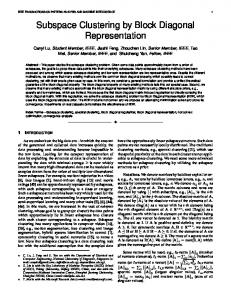
We evaluate the ability of our algorithm to detect and to construct a signature for different anomalies located in the same real traffic trace from the public MAWI repository of the WIDE project [2]. The WIDE operational network provides interconnection between different research institutions in Japan, as well as connections to different commercial ISPs and universities in the U.S.. The traffic repository consists of 15 minutes-long raw packet traces collected daily since 1999. The network traffic we shall work on consist of traffic from one of the trans-pacific links between Japan and the U.S., captured at sample point B. Reference [21] provides fragmented documentation for the whole data set. ICLA phase results for destination IP address /24 aggregated data are displayed on figure 3.(a). Each vertex is a cluster found in any of the generated sub-spaces. Each vertex number is the index of a cluster among the whole cluster set within the clustering ensemble P. The normal traffic is represented by the vertex group with the highest number of vertices. Every other group of points is a clique and potentially contains an anomaly. Figure 3.(b) depicts the outlier similarity graph obtained for destination IP address /24 aggregated data during the IOA phase. Each vertex number is the index of the associated outlier among the whole outlier set within the clustering ensemble P. The same graphs are built over the source IP address /24 aggregated data. Every edge means that the linked clusters or outliers are similar according to the criteria defined in III-B2. Every connected component which is also a clique is then extracted from the graph, considered as a potential anomaly. Each potential anomaly is assigned an index. This index has the following meaning: values between 0 and 99 means anomalies from clusters found in source IP address aggregated data, values between 100 and 199 means anomalies from outliers found in source IP address aggregated data, values between 200 and 299 means cluster found in destination IP address aggregated data and values between 300 and 399 means anomalies from outliers found in destination IP address aggregated data. The choice of 100 anomalies for each type of anomaly source is made under the assumption that there is less than 100 cliques in each graph. Once anomalies are extracted from feature spaces by the unsupervised detection, we apply anomaly correlation in order to find flows that are different from the normal ones in both aggregation type: source IP address and destination IP address. Figure 3.(c) depicts the anomalies similarities as a graph. Anomaly correlation then extracts three edges from the graph. Each edge represents the link between two similar anomalies, here anomalies 101 and 300, 111 and 305, and finally 100 and 205.

10

66

105

71

38

47

47

7

58

91 102

45

54

59 32 22

8

85

36

73 40

13 108

7

83

32 80 19 60 104 11 99 95 68 106

109 88

41

0

55

55

63 34

61 8 33 5 46 63 42 2 79 64 48 53

65

24

10

75 43

52

16 89

2

14

58

4

(a) Cluster similarity graph

Fig. 3.

52

35

6

205

49

111

28 90

82

17

100

26 9

3

39

20

21

25

38

86

113

101

97

62

305

72

103 112 100 96 71 107

18

17

30

51 74 29 70 31 66 77 57 76

43

67

14 0

45

11

69 37

15

92

41

35556 3 6 42 5 2 0 1 9 27 6 86 9 1 2 2 1 5 3 4 93 9 3 73 15 0 3 07 6 7 2 2 9 19 6 0 4 0 1 5 4 8 6412 2 34 4 46 33 6

94

98

67

57

54

56

93

73

26

87

27

23

28

16

70

4

22

78

24

123

62 36

75

18

115 1

65

59

101

34 111

84

12 110

81

44

(b) Outlier similarity graph

300

(c) Anomaly similarity graph.

Cluster similarity graph and outlier similarity graph for destination aggregated data. Anomalies are easily identified through cliques. TABLE II S IGNATURES OF ANOMALIES FOUND . Source traffic segment indice 111 112 100

Anomaly type Few ICMP pkts Few ICMP pkts Network scan

Destination traffic segment indice 305 309 205

1

1

0.9

0.9

0.8

0.8

absolute filtering rule

0.6 relative filtering rule

0.5 0.4 0.3

0.1

Fig. 4. MAWI.

VIII. C ONCLUSIONS absolute filtering rule

50

100

150 nDsts

200

250

0.6

relative filtering rule

0.5 0.4 0.3

Cluster 1 Cluster 2 Cluster 3 Anomalous flows Outliers

0.2

0 0

Destination signature nSrcs = 1, nICMP/nPkts > λ2 nSrcs = 1, nICMP/nPkts > α2 nSrcs = 1, nDsts > β3 , nSYN/nPkts > β4

0.7 nSYN/nPkts

nSYN/nPkts

0.7

Source signature nSrcs = 1, nICMP/nPkts > λ1 nSrcs = 1, nICMP/nPkts > α1 nSrcs = 1, nDsts > β1 ,nSYN/nPkts > β2

Cluster 1 Cluster 2 Anomalous flows Outliers

0.2 0.1 300

0 0

200

400

600 800 nSrcs

1000

1200

1400

Filtering rules for characterization of the found network scan in

Table II details each anomaly with its type, the segment indices extracted from ICLA and IOA and the two signatures detected from both source and destination aggregated data. The terms “Few ICMP packets” actually means that these two anomalies were containing just a few harmless ICMP packets. Both of these anomalies could have easily been discarded by an impact estimation based on nPkts/second. Figures 4.(a,b) depicts the results of the characterization phase for a network scan anomaly. Each sub-figure represents a partition Pn for which filtering rules were found. They involve the number of IP sources and destinations, and the fraction of SYN packets. Combining them produces a signature that can be expressed as (nSrcs == 1) ∧ (nDsts > λ1 ) ∧ (nSYN/nPkts > λ2 ), where λ1 and λ2 are two thresholds obtained by separating normal and anomalous clusters at half distance. This signature makes perfect sense: the network scan uses SYN packets from a single attacking host to a large number of victims. The main advantage of the unsupervised approach relies on the fact that this new signature has been produced without any previous information about the attack or the baseline traffic.

The completely unsupervised anomaly detection algorithm we have presented has many interesting advantages w.r.t. previous proposals in the field. It uses exclusively unlabelled data to detect and characterize network anomalies, without assuming any kind of signature, particular model, or canonical data distribution. This allows to detect new previously unseen anomalies, even without using statistical-learning or human analysis or decision making. Despite using ordinary clustering techniques, the algorithm avoids the lack of robustness of general clustering approaches by combining the notions of Sub-Space Clustering/Sub-Space Clustering, Inter-Cluster Association & Anomaly Correlation for Unsupervised Network Anomaly Detection and Anomaly Correlation. The characterization approach permits the construction of easy-to-interpretand-to-visualize results, providing insights and explanations about the detected anomalies to the network operator. We have evaluated the computational time of our algorithm. Results confirm that the use of the algorithm for on-line unsupervised detection and characterization is possible and easy to achieve for the volumes of traffic that we have analysed. Even more, they show that if run in a parallel architecture, the algorithm can reasonably scale-up to run in highspeed networks, using more traffic descriptors to characterize network attacks. We have verified the effectiveness of our proposal to detect and isolate distributed network anomalies on real traffic, in a completely blind fashion, without assuming any particular traffic model, significant clustering parameters, or even clusters structure beyond a basic definition of what an anomaly is. This provides a strong evidence of the accuracy of the

SSC-ICLA/IOA-Anomaly Correlation-based method to detect network anomalies. We think that this approach constitute a great step toward an autonomous network anomaly detection that will allow networks to self-diagnose themselves and thus faster reactions and lower operational costs. ACKNOWLEDGMENTS This work has been done in the framework of the ECODE project, funded by the European commission under grant FP7ICT-2007-2/223936. R EFERENCES [1] J. Mazel, P. Casas, and P. Owezarski, “Sub-space clustering & evidence accumulation for unsupervised network anomaly detection,” ser. TMA ’11, 2011. [2] K. Cho, K. Mitsuya, and A. Kato, “Traffic data repository at the wide project,” ser. ATEC ’00, pp. 263–270. [Online]. Available: http://portal.acm.org/citation.cfm?id=1267724.1267775 [3] P. Barford, J. Kline, D. Plonka, and A. Ron, “A signal analysis of network traffic anomalies,” ser. IMW ’02. [Online]. Available: http://doi.acm.org/10.1145/637201.637210 [4] J. D. Brutlag, “Aberrant behavior detection in time series for network monitoring,” in Proceedings of the 14th USENIX conference on System administration, 2000, pp. 139–146. [Online]. Available: http://portal.acm.org/citation.cfm?id=1045502.1045530 [5] A. Lakhina, M. Crovella, and C. Diot, “Diagnosing network-wide traffic anomalies,” ser. SIGCOMM ’04, pp. 219–230. [Online]. Available: http://doi.acm.org/10.1145/1015467.1015492 [6] ——, “Mining anomalies using traffic feature distributions,” ser. SIGCOMM ’05, pp. 217–228. [Online]. Available: http://doi.acm.org/ 10.1145/1080091.1080118 [7] A. Soule, K. Salamatian, and N. Taft, “Combining filtering and statistical methods for anomaly detection,” ser. IMC ’05. [Online]. Available: http://portal.acm.org/citation.cfm?id=1251086.1251117 [8] B. Krishnamurthy, S. Sen, Y. Zhang, and Y. Chen, “Sketch-based change detection: methods, evaluation, and applications,” ser. IMC ’03, pp. 234– 247. [Online]. Available: http://doi.acm.org/10.1145/948205.948236 [9] G. Dewaele, K. Fukuda, P. Borgnat, P. Abry, and K. Cho, “Extracting hidden anomalies using sketch and non gaussian multiresolution statistical detection procedures,” ser. LSAD ’07, pp. 145–152. [Online]. Available: http://doi.acm.org/10.1145/1352664.1352675 [10] F. Silveira and C. Diot, “Urca: Pulling out anomalies by their root causes,” ser. INFOCOM ’10, pp. 1–9. [11] L. Portnoy, E. Eskin, and S. Stolfo, “Intrusion detection with unlabeled data using clustering,” ser. DMSA-2001, pp. 5–8. [12] E. Eskin, A. Arnold, M. Prerau, L. Portnoy, and S. Stolfo, “A geometric framework for unsupervised anomaly detection: Detecting intrusions in unlabeled data,” in Applications of Data Mining in Computer Security, 2002. [13] K. Leung and C. Leckie, “Unsupervised anomaly detection in network intrusion detection using clusters,” ser. ACSC ’05, pp. 333– 342. [Online]. Available: http://portal.acm.org/citation.cfm?id=1082161. 1082198 [14] L. Parsons, E. Haque, and H. Liu, “Subspace clustering for high dimensional data: a review,” SIGKDD Explor. Newsl., vol. 6, pp. 90–105, June 2004. [Online]. Available: http://doi.acm.org/10.1145/ 1007730.1007731 [15] A. L. N. Fred and A. K. Jain, “Combining multiple clusterings using evidence accumulation,” IEEE Trans. Pattern Anal. Mach. Intell., vol. 27, pp. 835–850, June 2005. [Online]. Available: http://dx.doi.org/10.1109/TPAMI.2005.113 [16] G. Cormode and S. Muthukrishnan, “What’s new: finding significant differences in network data streams,” Networking, IEEE/ACM Transactions on, vol. 13, pp. 1219 – 1232, 2005. [17] G. Fernandes and P. Owezarski, “Automated classification of network traffic anomalies,” in Proceedings SecurComm’09, 2009. [18] A. K. Jain, “Data clustering: 50 years beyond k-means,” Pattern Recognition Letters, vol. 31, pp. 651–666. [Online]. Available: http://linkinghub.elsevier.com/retrieve/pii/S0167865509002323

[19] A. Strehl and J. Ghosh, “Cluster ensembles — a knowledge reuse framework for combining multiple partitions,” J. Mach. Learn. Res., vol. 3, pp. 583–617, March 2003. [Online]. Available: http://dx.doi.org/10.1162/153244303321897735 [20] R. Agrawal, J. Gehrke, D. Gunopulos, and P. Raghavan, “Automatic subspace clustering of high dimensional data for data mining applications,” ser. SIGMOD ’98, pp. 94–105. [Online]. Available: http://doi.acm.org/10.1145/276304.276314 [21] R. Fontugne, P. Borgnat, P. Abry, and K. Fukuda, “Mawilab: combining diverse anomaly detectors for automated anomaly labeling and performance benchmarking,” ser. Co-NEXT ’10, pp. 1–12.