Suitability of Markov Random Field-Based Method for Super ...

Kassaye, Geoinfor Geostat: An Overview 2013, S1 http://dx.doi.org/10.4172/2327-4581.S1-012

Geoinformatics & Geostatistics: An Overview

Research Article

Suitability of Markov Random Field-Based Method for Super-Resolution Land Cover Mapping

a SciTechnol journal different phenomena. MRF has been used in remote sensing data for several applications; for example: super-resolution land cover mapping [7], change detection [8] and multisource data fusion [4,9]. This study is concerned in assessing the suitability of the MRF-based approach for super-resolution land cover mapping.

Objective

Rahel Hailu Kassaye1*

The objective of this research is to assess MRF based SRM method suitability for land cover mapping and identify the influence of the method parameters on the quality of MRF based SRM.

Abstract

Structure of the paper

Super-resolution mapping (SRM) works by dividing the coarse pixel into sub-pixels and assign the class proportion estimated by subpixel classification to each corresponding sub-pixels then the class labelling is optimized based on the principle of spatial dependency. Among the existing SRM techniques Markov random field (MRF)based SRM is one of the most recently introduced technique. This study attempts to assess the suitability of the technique for superresolution land cover mapping. The spatial contextual smoothness constraint and spectral information were modelled with prior energy and the likelihood energy function respectively. These two energy functions were balanced with a smoothing parameter. Parameterization was done using the synthetic data sets and the effect of several factors on the quality of SRM was observed. The main findings in this study are: increasing the neighbourhood size while increasing scale factor enables to keep the Markovian property and the variability of optimal smoothing parameter in relation to the class separability. The appropriate setting of the optimal smoothing parameter can give a reasonable accuracy even for classes with low separability. The research result from both data sets proof the suitability of the method for super-resolution land cover mapping.

The introduction part of the paper highlights the background and objectives of the research. In the second part, the method employed in this study presented, the third part discusses the data type used, and then the result of the study and discussion has been presented on the fourth part of the paper. Finally, the conclusion has been drawn.

Keywords SRM; MRF; Neighbourhood; Class separability; Scale factor; Smoothing parameter

Introduction Background Super-resolution mapping (SRM) is a technique that transforms a soft classification result into a finer scaled hard classification [1]. This can be accomplished by assuming spatial dependence [2,3], in which spatially closer pixels tend to be more alike than more distant ones. In SRM spatial dependency between and within pixels can be maximized by integrating spatial context. Spatial context is defined by the correlations between spatially adjacent pixels in spatially neighboring pixels [4]. The use of contextual information is indispensable for efficient image interpretation. Contextual information can be integrated for image analysis by using Markov Random Fields (MRFs) [5,6]. MRF theory is a branch of probability theory for analyzing the spatial or contextual dependencies of

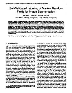
MRF-Based SRM Technique Super-resolution mapping technique Super-resolution mapping approach was accomplished by assuming spatial dependence, i.e. the tendency of neighboring pixels to have closer value than distant ones [2]. The key problem of subpixel mapping is determining the most likely locations of the fractions of each land cover class within the pixel. This works by dividing the large pixels with the corresponding scale factor which is defined as a ratio between the coarse and fine resolution pixels in the rows and columns direction to get sub-pixels; and the land cover is allocated to the latter, in such a way that spatial dependency is maximized. This leads to an artificial increase in spatial resolution and consequently an increase in data [1]. The illustrations in Figure 1a shows the coarse spatial resolution pixels, with associated proportion of one land cover class. Figure 1b and 1c denote the possible assignment of sub-pixels to that particular land cover class after the coarse pixels are divided by a scale factor of 5. The main advantage of this technique is that it will avoid losing important information the way conventional techniques do [2]. Therefore, super-resolution techniques would be useful to know where within the pixel, each class is located spatially.

Initial SRM generation The degraded coarse spatial resolution image and the fine spatial SRM are related by the scale factor. Suppose X be the degraded coarse spatial resolution image having M*N pixels and Y be the fine spatial resolution SRM having SM*SN pixels where S is the scale factor. That means a particular pixel in the coarse spatial resolution image

*Corresponding author: Rahel Hailu Kassaye, P.O. Box 3221, Addis Ababa, Ethiopia, Tel: +251-911-809-340, Fax: +251-115-540-630; E-mail: rhlhailu@ gmail.com, [email protected] Received: March 29, 2013 Accepted: July 12, 2013 Published: July 23, 2013

International Publisher of Science, Technology and Medicine

Figure 1: Super-resolution Mapping © Verhoeye et al (2002).

All articles published in Geoinformatics & Geostatistics: An Overview are the property of SciTechnol, and is protected by copyright laws. Copyright © 2013, SciTechnol, All Rights Reserved.

Citation: Kassaye RH (2013) Suitability of Markov Random Field-Based Method for Super-Resolution Land Cover Mapping. Geoinfor Geostat: An Overview S1.

doi:http://dx.doi.org/10.4172/2327-4581.S1-012 contains S2 pixels. The fraction image produced by applying linear spectral unmixing was an input for this algorithm. First each pixel was divided by the scale factor to get sub-pixels then each sub-pixel was randomly labeled with the corresponding classes from the coarse fraction image. The number of sub-pixels allocated to the given class can be expressed as n=fi*S2, where fi is the proportion of a given class in pixel i. Thus, n numbers of sub-pixels are randomly labeled by the given class. The expected output from this step was an SRM with many isolated pixels which further needs an iterative process to optimize the spatial dependence.

Optimization of the initial SRM The second phase was based on an optimization algorithm which can iteratively refine the initial super-resolution map by updating each pixel with the new class label to accurately characterize the spatial dependence between the class proportions of the neighboring pixels. Since, MRF model has a flexible framework for combinations of the contextual information from neighboring pixels and the information from the distribution of the data, the image was modeled by using MRF model. Two energy functions are defined to introduce both contextual constraint and spectral information as prior and likelihood energy respectively. These two energies are combined to yield a global energy. The smoothing parameter (λ) was introduced to use as a balancing factor between the two constraints. Then pixel labeling was accomplished by minimizing the energy function which is equivalent to maximizing the probability of labeling. Neighborhood system: For SRM the neighbourhood order should increase in relation to the scale factor so that all the sub-pixels present within the coarse pixel can be included in the neighbourhood system and this enables to keep the Markovian property within the neighbouring sub-pixels. Hence, we considered a neighbourhood size variable with the scale factor and the minimum neighbourhood order considered is second order or window size 3 for a scale factor of 2. To implement this growth of the neighbourhood size in relation to the scale factor (S) two relations were established and given by equations 1 and 2: Wsize = 2 * ( S − 1) + 1



Wsize = 2 * S + 1

(1) (2)

where; Wsize is the window size and 5 is the scale factor. Class separability: Class separability is a statistical measure indicating how well the classes can be separated during the classification process. The simplest class separability measure is the Euclidean distance, defined as the spectral distance between the mean vectors of each pair of signatures. If the spectral distance between two samples is not significant for any pair of bands, then they may not be distinct enough to produce a successful classification. The basic premise is that values within a given cover type should be close together in the measurement space, whereas data in different classes should be comparatively well separated [10]. The most commonly used statistical parameters for calculating class separability are a transformed divergence and a covarianceweighted distance between class means. Transformed divergence (TDij) is defined by equation 3. Because of its exponential character it can demonstrate the relation of classification accuracy with increasing class separation better than simple divergence [11]. Special Issue 1 • 012

  − Dij   TDij = 2 * 1 − exp     8   

(3)

where; Dij refers to divergence index between two classes i and j. Divergence measures the separability of probability distributions that has its basis in their degree of overlap [11]. Markov random field: In SRM spatial dependency between and within pixels can be maximized by integrating spatial context. Spatial context is defined by the correlations between spatially adjacent pixels in a spatially neighboring pixel [4]. The use of contextual information is indispensable for efficient image interpretation. Contextual information can be integrated for image analysis by using Markov Random Fields (MRFs) [5,6]. A Markov random field (MRF) is a random field which shows the following properties with respect to its neighborhood system [7]: • Positivity: P(x) > 0, when this condition is satisfied, the joint probability P(x) of any random field is uniquely determined by its local conditional probabilities; • Markovianity shows that labeling of a pixel is only dependent on its neighboring pixels, this can be described as: P(Xi | Xd-i)=P(Xi | XNi); • Homogeneity specifies the conditional probability for the label of a pixel, given the labels of the neighboring pixels, regardless of the relative location of the pixel; • Isotropy describes the independence of direction that means the neighboring pixels of the same order surrounding a given pixel have the same contributing effect to the labeling of the given pixel. Where; d−i refers to all the pixels in the set excluding the target pixel i and Ni denotes the neighbors to pixel i. For a random variable X is to be a Gibbs random field (GRF) on F with respect to the neighborhood N if and only if its configurations obey a Gibbs distribution in the following form: P (x) =

where;

 U (x) 1 * exp  −  Z  T 

(4)

 U (x) (5) Z = ∑ exp  −   T  is a normalization constant. Here we can define an energy function U(x), from equation 4 we can say that maximizing P(x) is equivalent to minimizing the energy function which can be formulated by the following equation: U ( x ) = ∑ c∈ Vc ( x )

(6)

Global energy construction: Suppose we have an image x with pixel gray values in a number of spectral bands, which are denoted by c, traditionally, each pixel is labeled based on a gray value alone without contextual information. When the context is introduced as prior information and modeled by means of MRF, Bayesian framework can be adopted to construct the global energy and labeling is carried out by minimizing this global energy, from equation 4, • Page 2 of 5 •

Citation: Kassaye RH (2013) Suitability of Markov Random Field-Based Method for Super-Resolution Land Cover Mapping. Geoinfor Geostat: An Overview S1.

doi:http://dx.doi.org/10.4172/2327-4581.S1-012 we can see that the lower the energy the higher is the probability of labeling. The Bayesian formula holds the following conditional probability relation:

P( x, c) = P(c | x) P( x) = P( x | c) P(c)

(7)

According to equation 4, Gibbs parameter was included as prior information in the construction of prior energy. The prior energy can be formulated as follows: U prior ( x i ) =

∑β

(8) where; β is a pair wise clique potential parameter and C is the clique in {i , j}∈C

the neighborhood system. The potential function for pair-wise cliques can be written as:  − β if i = j  β otherwise

β ( i, j ) = 

(9)

The single site clique was not considered here, because the probability of each class was considered to be the same and thus set to 0 as most applications do. Since this study was not dealing with texture, all the estimated Gibbs potential parameters were positive. Clique potential parameters were required in the iteration phase for prior energy computation, thus, proper estimation was very essential. Simulated annealing: Simulated annealing (SA) is a type of stochastic iterative optimization technique which is based on the use of random numbers and probability statistics for the global optimization problem. The concept of annealing is based on the manner in which liquids freeze or metals recrystallize in the process. The process which is initially at high temperature and disordered, is slowly cooled and the system becomes more ordered and approaches a frozen state as cooling proceeds. This process is controlled by the annealing parameters; these are initial temperature (T0) and updating schedule (Tupd). The parameter “temperature” is used to control the randomness of the optimization algorithm. High temperature indicates high randomness and low temperature indicates less randomness. This means that a high temperature can increase the probability of a pixel label being replaced by new class label even though the energy of the new class is higher. When the temperature decreases according to the predefined cooling schedule (T=T0 * Tupd), only small increase of energy is allowed. Increase of energy cannot be accepted, when it reaches to a freezing point, in other words there is no more pixel updating. The pixel updating was performed in a row wise scheme. To carry out this, the energy difference was defined as follows:

(

∆ = (i, j ) – i ' − j '

)

(10)

If ∆ > 0 then (i, j) can be replaced by new class label (i’,j’). In this research, the iteration was repeated three times for each temperature update value, if there is no change in pixel labeling in all the three iterations the algorithm was allowed to finish the process. Accuracy assessment: One of the quality measures that can be derived using the whole error matrix information is the kappa coefficient. This measure estimates the overall agreement between image data and the reference data [12]. It incorporates the offdiagonal elements as a product of row and column margins as follows: N ∑ i=1 xii − ∑ i=1 xii ( xi+ * x + i ) r

K=

r

N 2 – ∑ i=1 xii ( xi+ * x + i ) r

Special Issue 1 • 012



(11)

where, K is the estimated kappa coefficient, N is the total number of pixels in the image, r denotes the number of rows and columns in a confusion matrix and xi+ and x+i are the marginal total of row i and column j respectively. The kappa coefficient is always less than or equal to 1. The level of kappa can be interpreted differently as to what is a good level of agreement. A kappa coefficient of 1 means a perfect agreement with the reference data where as 0 means different from the actual value. The value of 0.7 or higher is generally regarded as good correlation, but of course, the higher the value is the better the correlation [12].

Data Sets and Preprocessing Data sets The data sets used in this research are the synthetic images and the remote sensing data. Synthetic image has been used in this study due to the fact that the exact end-member fractions can be defined. The generated synthetic image is multispectral with three bands. This is because the nonlinear interactions among end-members do not exist and exact class statistics information is known and does not have to be estimated. Furthermore, these images lack co-registration errors between the lower and the higher resolution images and visual checking of the method’s performance is easy on these images as they represent simple geometric features. Therefore, these images are used to set the parameters and study its influence on the quality of the output. For real data on the contrary, usually no good reference exists because co-registration at sub-pixel level is problematic and often there is a time-lag between high and low resolution images. The remote sensing data applied to test the method is IKONOS image; this image can yield relevant data for nearly all aspects of environmental studies. The image covers part of the Enschede area, in The Netherlands and it was acquired in April 03, 2000.

Preprocessing Image degradation model: The image degradation model down scaled the image by resampling fine pixels to the given scale to make up the new coarse pixels. This process facilitates comparison between fine and coarse resolution images. In this research the model followed a simple averaging technique by an integer factor in the X and Y direction. Following the mentioned image degradation model, the degraded images were prepared through down sampling of the fine resolution image with a given factor. This process was carried out for both synthetic and remote sensing images. These degraded images were used as an input for the spectral unmixing process. Spectral unmixing: The proportions of the classes within the synthetic image were estimated by applying linear spectral unmixing approach. It was constrained for the sum of the proportions to be a unity. This was performed by extracting the class mean and covariance information from the training sets. If class proportions are estimated accurately optimization takes less time but this point is not very critical. The output from the unmixing algorithm was a set of fraction images that shows the proportion of each class and this was an input for initial SRM generator algorithm.

Results and Discussion Proper parameters identification was the most crucial part of this study because a good choice of parameters can successfully lead • Page 3 of 5 •

Citation: Kassaye RH (2013) Suitability of Markov Random Field-Based Method for Super-Resolution Land Cover Mapping. Geoinfor Geostat: An Overview S1.

doi:http://dx.doi.org/10.4172/2327-4581.S1-012 to a good result. For this reason, the research aimed in searching the optimal parameters where high quality SRM can be found. The parameters which need to be determined were the neighbourhood size and smoothing factor (λ). From the experimental results of optimizing this annealing parameter, it is clear that at Tupd=0.8 higher mean kappa values can be found. For synthetic image2 setting Tupd=0.9 can also give a closer kappa value which is found at Tupd=0.8 but the number of iterations required for convergence were more than the required iterations at 0.8. Therefore, Tupd=0.8 can be considered optimal for low complex scenes and when the scene is more complex (for example, number of classes in the image) Tupd can be set to 0.9 for a slow temperature drop. Neighborhood size determination: To choose the appropriate size a comparison was made on the qualities of SRMs from three neighbourhood sizes. The first one was a second order neighbourhood size fixed for all scale factors. The second and the third were neighbourhood sizes variable with a scale factor. Following the established relationship of the window size, the number of neighbouring pixels (Nn) for the central pixel will be: Nn=(Wsize)2 − 1. Then all the sub-pixels which were in a given coarse pixel can be included as neighbouring pixels even when a corner subpixel is becoming a central pixel. But the neighbours up to second order show the eight pixels surrounding the central pixel this means some of the sub-pixels can be easily excluded from the neighbourhood system for large scale factors (Figure 2).

The effect of smoothing parameter The effect of smoothing factor (λ) has been attempted to be observed at various class separability level ranging from TD=0.5 to TD=1.9. The result from synthetic image1 demonstrated that, λ does not have a significant effect on the quality of SRM at variable class separability, as shown in (Figure 3a) all have a kappa value above 0.9 attribute to the absence of corner pixels, best quality contextual information case. In the case of synthetic image2 (Figure 3b), the plots for TD=1.5 and 1.9 show almost a similar pattern, the kappa value was increasing for a value of λ ranging from 0.4 to 0.2. When TD=0.5 and 1.0 the result shows a small drop where λ value is below 0.1. In general, the greater the value of (TDij), the greater is the

Note: the scale of the two plots is different. Figure 3: The effect of λ on the accuracy of SRM (a) on synthetic image1 (b) on synthetic image2.

class separability or the statistical distance between classes. A poor separability is indicated by a value of (TDij) smaller than 1.9 [13]. The probability of correct classification as a function of pair wise transformed divergence can be seen in Figure 3. In order to get the optimum result, one can set the values of λ ranging from 0.4 to 1 for a scene with homogeneous object and from 0.1 to 0.4 for a scene containing distributed objects, taking into account the class separability.

The effect of scale factor on the optimized SRM The accuracy of SRM versus the corresponding scale factor is shown with the error bars indicating the standard deviation of the accuracy values for both initial and optimized SRMs in Figure 4. The accuracy of both initial and optimized SRMs is decreasing with increasing scale factor value. At scale factor 6 the optimization doesn’t bring a significant improvement compared to the initial SRM. The observed decrease of the SRM quality with increasing scale factor value is due to the fact that the number of sub-pixels within the coarse resolution pixel increases fast with scale factor, making the coarse pixel to be highly mixed. The single observed spectral value for the coarse resolution pixel on one hand side and many possible sub-pixel configurations with equivalent contextual energy on the other hand side make the problem strongly underdetermined.

SRM results from remote sensing data sets The initial SRMs contain many isolated pixels and therefore have a noisy appearance. To get smooth SRMs with correctly labeled pixels the MRF-based SRM optimization needs to be applied on the initial SRMs. Since the value of class separability varies from 1.9 to 2.0, the smoothing parameter λ was set to a value of 0.4. Then, the optimized SRM with better quality was generated for each scale factor after an iterative optimizing process. The reference map and the output of the method for a scale factor (S) values 2, 3 and 4 are displayed in Figure 5 from top to bottom respectively.

Conclusion

Figure 2: The neighborhood size determination, Black: Wsize = 2 * (S − 1) + 1, Red: Wsize = 2 * S + 1 and Blue: Wsize = 3.

Special Issue 1 • 012

One of the major findings of this study is that the MRF-based SRM method can produce a better quality SRM when the neighborhood size grows in relation to the scale factor than a fixed second order neighborhood size. If the proper smoothing parameter is not assigned properly either there could be an over smoothing effect because of ignoring spectral information and giving more weight to the contextual information when it is set above the optimal value or there could be a noisy appearance when it is set below the optimal value • Page 4 of 5 •

Citation: Kassaye RH (2013) Suitability of Markov Random Field-Based Method for Super-Resolution Land Cover Mapping. Geoinfor Geostat: An Overview S1.

doi:http://dx.doi.org/10.4172/2327-4581.S1-012 SRM would not have better quality than the initial SRM. Therefore, the capability of the method to cope with the complexity of the scene and to multiple land cover classes has been examined and the results demonstrate the potential of the MRF-based method for super-resolution land cover mapping application. Acknowledgements I would like to thank the Netherlands government and ITC for awarding NFP scholarship for this study. I am also very grateful to Dr. V.A. Tolpekin and Dr. Ir. W. Bijker for their continuous guidance and advice.

References 1. Verhoeye J, RD Wulf (2002) Land cover mapping at sub-pixel scales using linear optimization techniques. Remote Sensing of Environment 79: 96-104. Figure 4: The effect of scale factor on the quality of SRM; Blue: Initial, SRM Black: Optimized SRM.

2. Atkinson PM, Cutler MEJ, Lewis H (1997) Mapping sub-pixel proportional land cover with AVHRR imagery. International Journal of Remote Sensing 18: 917–935. 3. Mertens KC, Verbeke LPC, Ducheyne EI, Wulf RRD (2003) Using genetic algorithms in sub-pixel mapping. International Journal of Remote Sensing 24: 4241-4247. 4. Solberg AHS, Taxt T, Jain AK (1996) A Markov random field model for classification of multisource imagery. IEEE Trans. Geoscience and Remote Sensing 34:1. 5. Li SZ (2001) Markov random field modelling in image analysis. Springer. 6. Tso B, Mather P (2001) Classification Methods for Remotely Sensed Data. CRC Press. 7. Kasetkasem T, Arora MK, Varshney PK (2005) Super-resolution land cover mapping using a Markov random field based approach. Remote Sensing of Environment 96: 302–314. 8. Kasetkasem T, Varshney PK (2002) An image change detection algorithm based on Markov random field models. IEEE Transactions on Geoscience and Remote Sensing 40: 1815-1823. 9. Sarkar A, Banerjee A, Banerjee N, Brahma S, Kartikeyan B, et al (2005) Landcover Classification in MRF Context Using DempsterShafer Fusion for Multisensor Imagery. IEEE Trans Image Process 14: 634-45. 10. Erdas Field Guide (4thedn) Atlanta, Georgia. 11. Richards JA (1993) Remote sensing digital image analysis: An introduction (2nd edn.) Springer-Verlag. 12. Rusell GC (1991) A review of assessing the accuracy of classifications of remotely sensed data. Remote Sensing Environment 37: 35-46. 13. Lilles TM, RW Kiefer, J Chipman (2004) Remote sensing and image interpretation (5th edn.) Wiley and Sons.

Figure 5: MRF-based SRM output from S = 2 to S = 4, from left to right are input image, initial SRM and optimized SRM respectively.

due to the low weight given to the neighbouring pixel information. According to the experimental results, when the scene contains homogeneous objects and distributed objects the parameter λ can be set to a value ranging from 0.4 to 1.0 and 0.1 to 0.4 respectively. The quality of SRM decreases with increasing the scale factor. The reason for this is that the number of sub-pixels within the coarse resolution pixel increases fast with scale factor, making the coarse pixel to be highly mixed. The class separability is more significant with increasing the number of classes so that the smoothing parameter should be set strictly at the optimal value otherwise the optimized Special Issue 1 • 012

Author Affiliation 1

Top

Ministry of Urban Development & Construction, Addis Ababa, Ethiopia

Submit your next manuscript and get advantages of SciTechnol submissions ™™ ™™ ™™ ™™ ™™ ™™ ™™

50 Journals 21 Day rapid review process 1000 Editorial team 2 Million readers More than 5000 Publication immediately after acceptance Quality and quick editorial, review processing

Submit your next manuscript at ● www.scitechnol.com/submission

• Page 5 of 5 •